Computer Graphics: Materials
Materials
This report explains the fundamental concepts of implementing various materials—diffuse, metallic, and dielectric-in a ray tracing renderer.
Ray Tracing
- Before diving into the materials, it is crucial to understand the core principles of ray tracing at first.
Forward vs. Backward Path Tracing
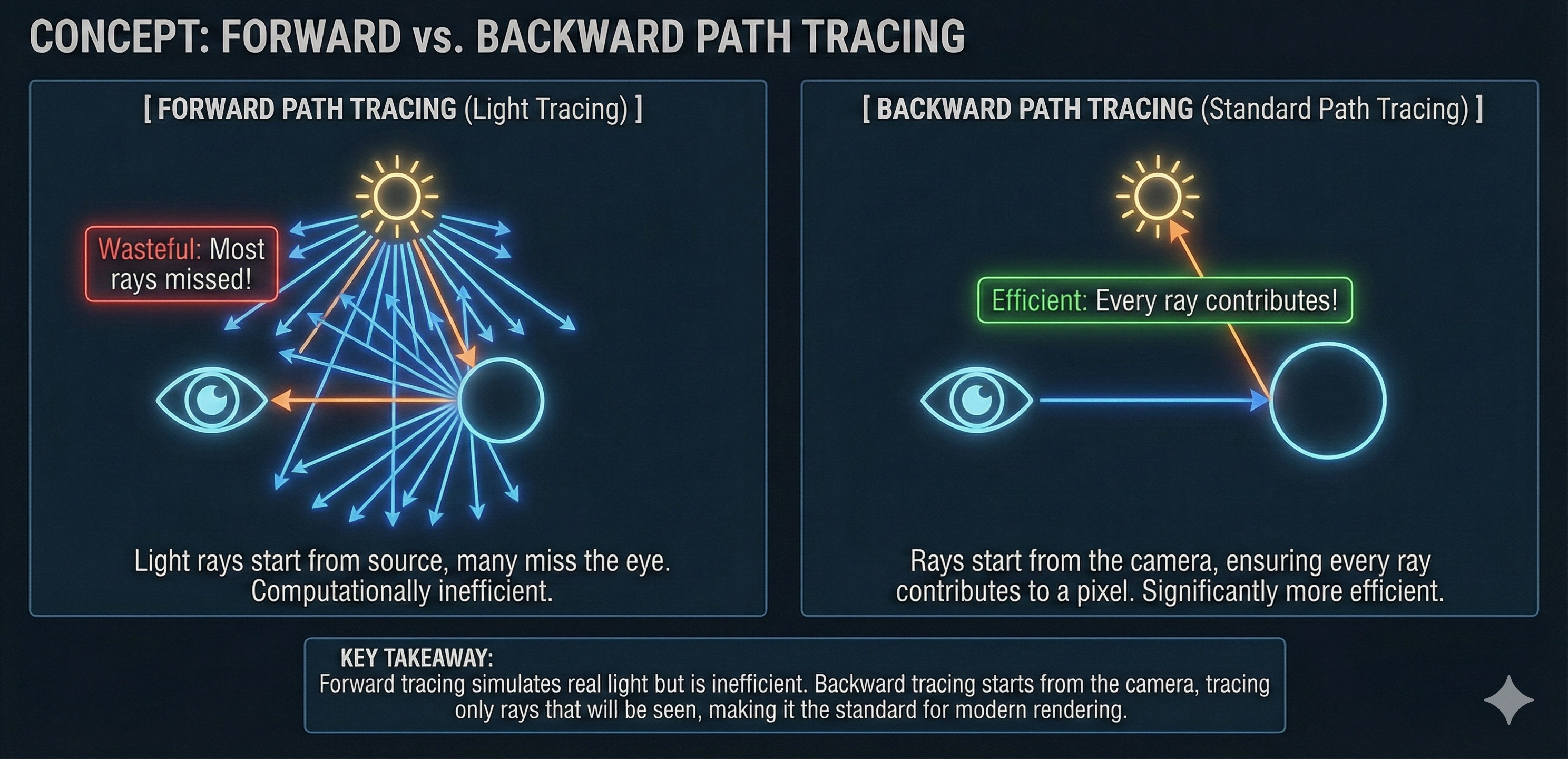
- In the real world, light rays originate from light sources and travel through a scene, bouncing off surfaces until they reach an observer’s eye.
- This process is known as light tracing or forward path tracing.
- However, directly simulating this is computationally inefficient.
- Only a minuscule fraction of the light rays emitted from a source will ever reach the camera, resulting in wasted computation.
- While forward path tracing can be effective for specific scenarios like rendering caustics, most modern ray tracers use a different approach.
- Backward path tracing (or simply “path tracing”) works in the opposite direction.
- It casts rays from the camera (or eye) into the scene.
- This approach is significantly more efficient.
- Because it ensures that every ray calculated contributes to a visible pixel on the screen.
- In this model, a ray is traced from a pixel on the camera’s sensor into the scene.
- If the ray intersects an object, a new ray is scattered from that intersection point.
- This process continues recursively until the ray either hits a light source, or a maximum bounce limit is reached.
- If the ray ultimately hits a light source,
- it carries a contribution of that light’s color back to the camera, which is then attenuated by the properties of each surface it interacted with.
- If the ray never hits a light,
- it is assigned a default background color (often black).
- If the ray intersects an object, a new ray is scattered from that intersection point.
Diffuse Albedo
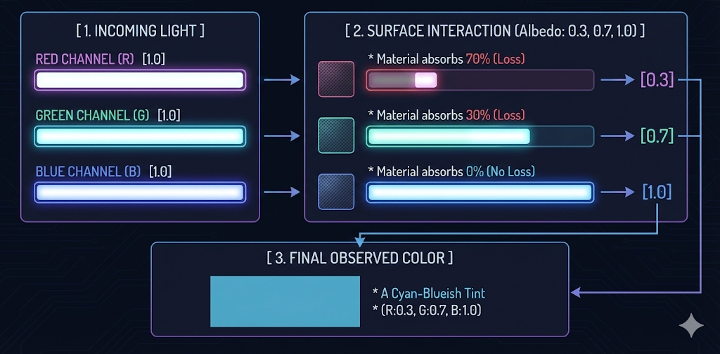
- The diffuse albedo is a material property that defines the percentage of incoming light that a surface reflects uniformly in all directions.
- For example, a surface with an albedo of $[0.3, 0.7, 1.0]$ will absorb $70\%$ of the red, $30\%$ of the green, and $0\%$ of the blue components of the incoming light.
- The remaining light, modulated by the albedo, is what gives the object its color.
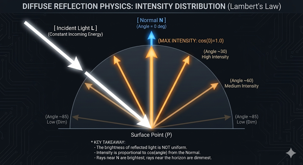
Light Intensity
- The intensity of light received by a surface depends on the angle between the surface normal and the incoming light ray.
- The maximum intensity is achieved when the light ray is parallel to the surface normal, and it decreases as the angle increases.
-
This relationship is described by Lambert’s Cosine Law.
\[I_\text{reflected} = I_\text{original} * cos\theta\]- The angle $\theta$ is the angle between the surface normal and the incoming light ray.
- The intensity is typically constrained to be non-negative by utilizing a function such as $max(0,cos\theta)$.
Recursive Calculation
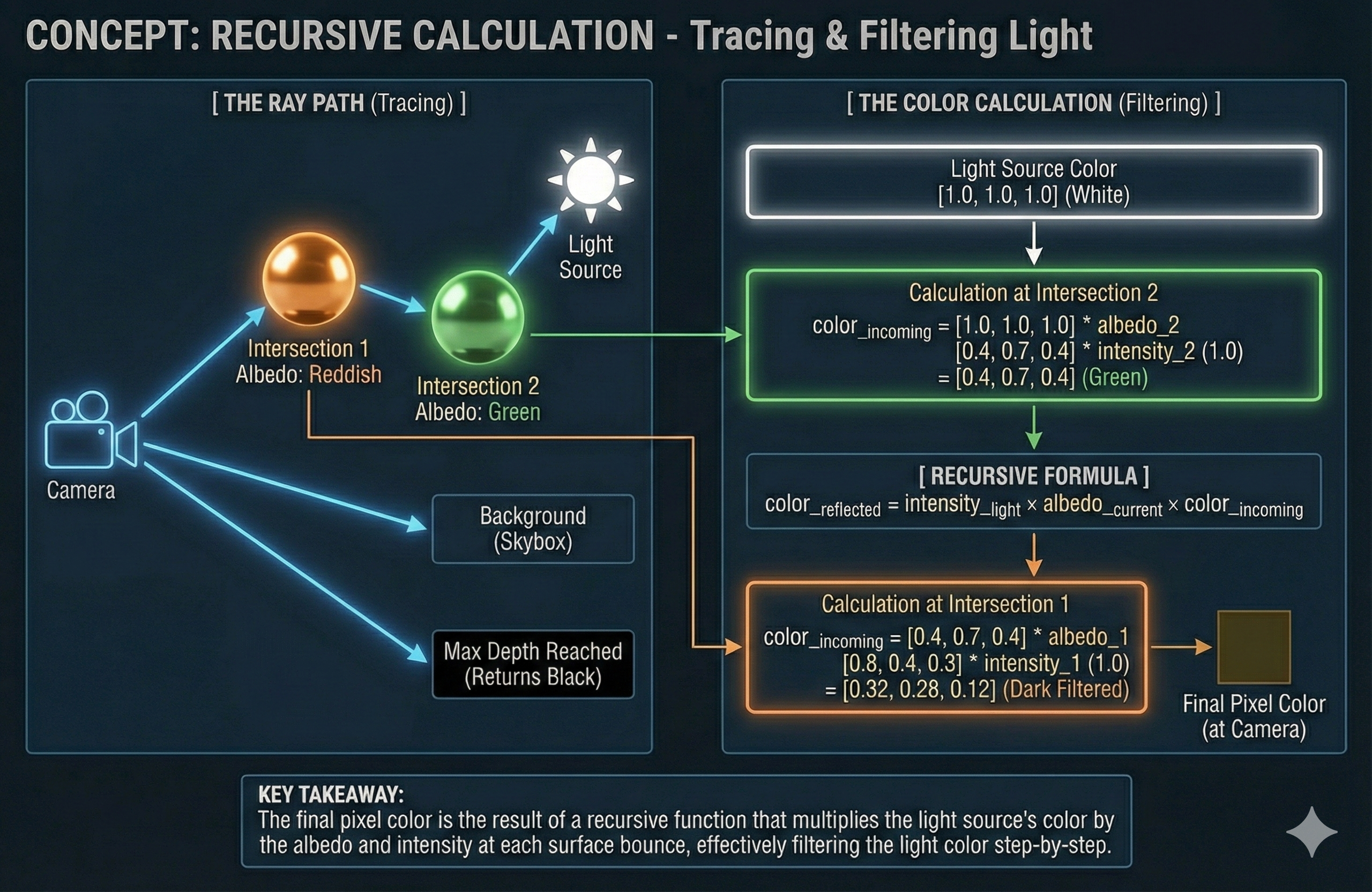
- To calculate the final color of a pixel, ray tracers use a recursive function.
- A ray is traced from the camera, and at each bounce, the color is determined by a product of the surface’s properties and the color from the subsequent ray.
-
The core recursive formula can be generalized as:
\[\text{color}_{\text{reflected}} = \text{intensity}_{\text{light}} \times \text{albedo}_{\text{current}} \times \text{color}_{\text{incoming}}\]- This formula describes a series of modulations.
- Initially, the color of the incoming ray is multiplied by the diffuse albedo of the intersected surface.
- This multiplication simulates the absorption and reflection of each RGB component.
- The result is then attenuated by the light intensity, a scalar value derived from the angle of incidence.
- The final product of these operations determines the color of the reflected ray.
- The recursion terminates in one of three cases:
- A ray hits a light source
- The recursion ends, and a color of light source (e.g., white) is returned.
- A ray hits nothing
- The recursion ends, and a background or skybox color is returned.
- The maximum recursion depth is reached
- The ray is assumed to have lost all its energy, and the function returns black.
- This is a crucial optimization to prevent infinite loops and limit computation.
- A common maximum depth is between 5 and 10 bounces.
- A ray hits a light source
-
Recursive Ray Tracing Path Illustrating Color Filtering.
Light Absorption and Filtering
- The color of a ray is not a constant value.
- It is a cumulative property that is filtered at each surface it interacts with.
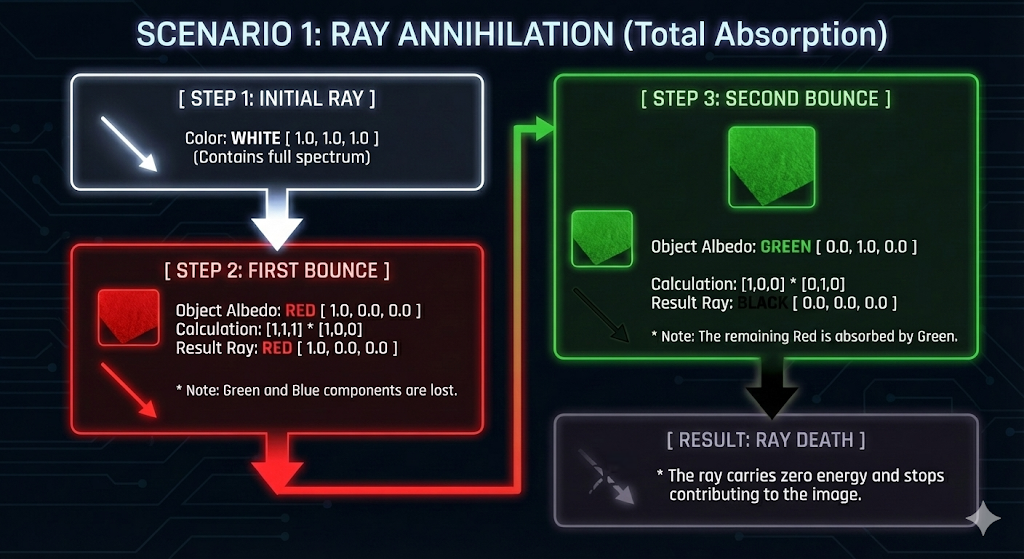
Scenario 1: Ray Annihilation
- A ray can effectively “die” if it is filtered by a surface that completely absorbs its color components.
- Initial state
- A white ray (RGB = $[1, 1, 1]$)
- Bounce 1
- The ray hits a pure red object (albedo $[1, 0, 0]$).
- The ray’s color becomes red, losing its green and blue components.
- Bounce 2
- The now-red ray hits a pure green object (albedo $[0, 1, 0]$).
- The object absorbs all red light, and since there are no green or blue components left in the ray, the ray’s color becomes black (RGB = $[0, 0, 0]$).
- The ray effectively dies and no longer contributes to the final image.
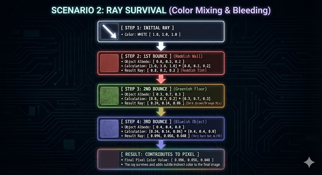
Scenario 2: Ray Survival
- If a ray’s color and an object’s albedo have overlapping color components, the ray can survive multiple bounces, albeit with reduced intensity.
- This is what creates complex and realistic colors.
- Initial state
- A white ray (RGB = $[1, 1, 1]$).
- Bounce 1
- Hits a reddish wall (albedo $[0.8, 0.2, 0.2]$).
- The ray becomes a reddish light.
- Bounce 2
- Hits a greenish floor (albedo $[0.3, 0.7, 0.3]$).
- The ray becomes a dimmer, mixed-color light.
- Bounce 3
- Hits a bluish object (albedo $[0.4, 0.4, 0.8]$).
- The ray’s final color is a very dim, mixed-color light.
- Initial state
-
The final pixel value is the cumulative result of all these color-filtering interactions, which is why a single ray’s journey through a scene is what determines the final pixel’s color.
Duality of Surface Form: Micro/Macro Space
- In rendering, the behavior of a surface is interpreted differently depending on the viewing scale.
-
This duality is fundamental to accurate shading.
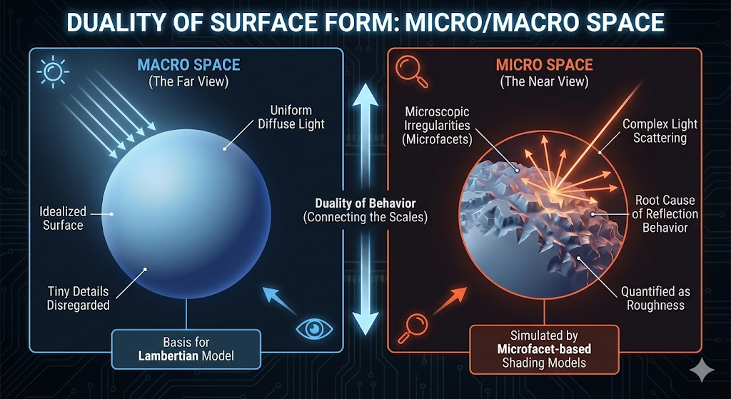
Macro Space (The Far View)
- Definition: This represents the surface appearance when viewed from a far distance.
- Behavior: The surface appears to be illuminated uniformly by Diffuse Light.
- Modeling: This view forms the basis for idealized shading models like the Lambertian model, where the surface’s tiny details are disregarded.
Micro Space (The Near View)
- Definition: This represents the actual surface when viewed at a close, microscopic level.
- Behavior: The physical surface possesses Microscopic Irregularities or Microfacets.
- These minute bumps and grooves are the root cause of light being scattered in an unpredictable manner.
- Representation: This scattering behavior is quantified and expressed as the material’s Roughness.
- Significance: Accurate, photorealistic rendering necessitates the simulation of these microscopic irregularities using complex Microfacet-based shading models.
- These advanced models account for the statistical orientation and geometry of these tiny facets to precisely predict light reflection.
Reflection in Ray Tracing
- Ray tracing simulates how light interacts with surfaces by calculating the paths of light rays.
- The behavior of these rays upon hitting an object depends on the object’s material properties.
- This section details the implementation of three fundamental reflection models
- diffuse (Lambertian)
- specular (Metal)
- and a combination of the two (Fuzzy Reflection).
Diffuse (Lambertian) Reflection
- Diffuse Reflection is a characteristic of matte, non-glossy surfaces.
- Mechanism: Light reaching the surface is scattered uniformly in all directions due to the surface’s Microscopic Irregularities. An ideal Lambertian surface appears to have the same brightness regardless of the observer’s viewpoint.
- Illumination Intensity: The surface’s brightness is proportional to the cosine of the angle between the incident light and the normal, as defined by Lambert’s Cosine Law.
- To accurately simulate diffuse reflection and solve the Rendering Equation, Ray Tracing employs Cosine-Weighted Hemisphere Sampling based on the Monte Carlo method.
- Weighting: This technique generates new reflected rays such that directions closer to the surface normal ($\vec{n}$) are assigned a higher probability (a greater weight).
- Efficiency: This is highly efficient because rays near the normal contribute more significantly to the total scene illumination. By concentrating samples in this critical region, the method reduces image Noise and significantly improves computational efficiency.
- Implementation Steps:
- Arbitrary Vector Generation and Unit Sphere Normalization:
- An arbitrary coordinate $(\mathbf{x}, \mathbf{y}, \mathbf{z})$ is generated within the range $[-1, 1]$.
- This vector is then normalized to yield a random direction vector ($\vec{v}_{\text{rand}}$) on the surface of the Unit Sphere.
- (Note on Stability): Points too close to the center are rejected to ensure numerical stability.
- Hemisphere Constraint Check:
- The reflected ray must be constrained within the Hemisphere defined by the surface normal $\vec{n}$.
- This constraint is verified by checking the Dot Product between the normal $\vec{n}$ and the generated vector $\vec{v}_{\text{rand}}$.
- Direction Correction:
- If the dot product is negative (indicating the ray is pointing into the surface’s interior), the randomly generated direction vector is reversed (the direction is flipped by applying a negative sign).
- This forces the ray to be directed outwards into the required hemisphere.
- Arbitrary Vector Generation and Unit Sphere Normalization:
-
This systematic procedure generates computationally efficient and physically plausible diffuse reflections.
Specular (Metal) Reflection
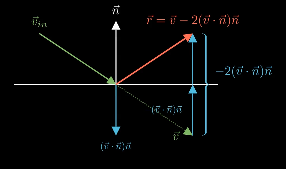
- Specular reflection occurs on polished, mirror-like surfaces where light is not scattered but is instead reflected in a single, predictable direction.
- The law of reflection states that the angle of incidence equals the angle of reflection.
-
The direction of a perfectly reflected ray can be calculated using the following formula, which is derived from vector mathematics:
\[v_\text{reflected}=v_\text{incident}−2(v_\text{incident}\cdot n)n\]- where:
- $v_{incident}$ is the normalized incoming light vector.
- $n$ is the normalized surface normal vector at the point of intersection.
-
The dot product ($v_{incident}\cdot n$) ensures the correct projection of the incident vector onto the normal, which is crucial for determining the reflected direction.
- where:
- For a dot product to correctly determine the reflection direction, it is essential that both the incident vector and the normal vector point away from the surface, or both point toward it.
- It’s standard practice to use the incoming ray direction (which points toward the surface) and an inverted normal vector for a consistent calculation.
-
Click to see the code
  inline Vec3 getReflectedMirror(const Vec3& inputVector, const Vec3 &unitVector) {
      return inputVector - 2 * performDot(inputVector, unitVector) * unitVector;
  }
Fuzzy Reflection
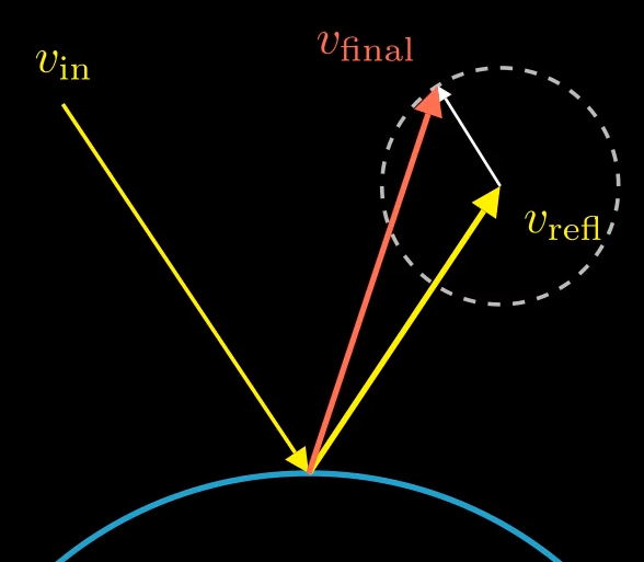
- Fuzzy reflection is a model for simulating less-than-perfectly-polished metallic surfaces, such as brushed or scuffed metals.
- This model introduces a degree of randomness to the specular reflection, scattering the reflected ray around the ideal specular direction.
- This effect is achieved by adding a small, random perturbation to the perfectly reflected ray vector.
- The magnitude of this perturbation is controlled by a fuzziness parameter, which effectively represents the radius of a sphere centered on the ideal reflection vector’s endpoint.
-
The formula for the scattered ray is as follows:
\[v_\text{scattered}=v_\text{unit_reflected}+f_\text{fuzziness}\cdot v_{\text{random}}\]- where:
- $v_\text{unit_reflected}$ is the normalized, perfectly reflected vector.
- $f_\text{fuzziness}$ is the scalar fuzziness parameter.
- $v_\text{random}$ is a random unit vector.
- where:
- An important implementation detail is ensuring that the scattered ray’s direction points outward from the surface.
- A simple check using the dot product between the scattered vector and the surface normal can be performed to absorb any rays that scatter back into the object.
-
Click to see the code
  class Metal : public Material {
  public:
      Metal(const Color& inputAlbedo, double inputFuzz) : albedo(inputAlbedo), fuzz(inputFuzz) {
          if (inputFuzz < -1)
              inputFuzz = -1;
          else if (inputFuzz > 1)
              inputFuzz = 1;
      }

      bool doesScatter(const Ray &inputRay, const HitRecord &record, Color &attenuation, Ray &scatteredRay) const override {
          Vec3 reflectedVector = getReflectedMirror(inputRay.getDirection(), record.normalizedVector);
          reflectedVector = getUnitVector(reflectedVector) + (fuzz * getRandomUnitVector());
          scatteredRay = Ray(record.hitPosition, reflectedVector);
          attenuation = albedo;
          return (performDot(scatteredRay.getDirection(), record.normalizedVector) > 0);
      }

  private:
      Color albedo;
      double fuzz;
  };
Refraction: The Behavior of Light in Dielectrics
- When a light ray encounters a dielectric—a transparent material like glass, water, or a diamond—it typically splits into two components:
- a reflected ray
- and a refracted (transmitted) ray.
- The reflected ray “bounces” off the surface, while the refracted ray passes into the material, bending its path due to a change in the speed of light.
Refractive Index (n) and Snell’s Law
- A material’s refractive index (n) is a dimensionless physical constant that quantifies how much light bends as it passes through it.
-
It is defined as the ratio of the speed of light in a vacuum (c) to the speed of light in the medium (v):
\[n={c\over v}\] -
The relationship between the refractive indices of two media and the angles of a light ray is governed by Snell’s Law:
\[n_1sin\theta_1=n_2sin\theta_2\]- Here, $\theta_1$ and $\theta_2$ are the angles of the incident and refracted rays, respectively, measured from the surface normal.
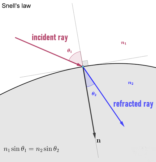
- When light enters a denser medium ( $n_1 < n_2$ ),
- it slows down and bends toward the normal.
- Conversely, when it enters a less dense medium ( $n_1 > n_2$ ),
- it speeds up and bends away from the normal.
- This law is fundamental for calculating the direction of a refracted ray in ray tracing, which is essential for rendering realistic transparent objects.
Calculating the Refracted Vector
- The direction of a refracted ray can be derived by decomposing the incident ray vector into components parallel and perpendicular to the surface normal.
-
For an incident unit vector $a$, a unit normal vector $n$, and a refracted unit vector $b$:
\[b = \frac{n_1}{n_2} (a - (a \cdot n) n) - \sqrt{1 - (\frac{n_1}{n_2})^2 (1 - (a \cdot n)^2)} \cdot n\] -
Click to see the full derivation
- The direction of a refracted ray can be mathematically derived using a vector approach based on Snell’s Law.
- The key is to decompose the incident and refracted vectors into components parallel and perpendicular to the surface normal.
- Let’s define our vectors:
- $a$: The normalized incident ray vector.
- $n$: The normalized surface normal vector.
- $b$: The normalized refracted ray vector.
- $\theta_1$: The angle between the incident ray and the normal.
- $\theta_2$: The angle between the refracted ray and the normal.
-
The incident and refracted vectors can be decomposed as follows:
\[a=a_{\parallel} + a_{\perp}\] \[b=b_{\parallel} + b_{\perp}\] - The magnitudes of the perpendicular components are related by Snell’s Law.
-
It’s possible to use the angles defined by the vectors and the normal
\[sin\theta_1= ||a_{\perp}||\] \[sin\theta_2= ||b_{\perp}||\]
-
-
Snell’s Law can then be expressed in vector form:
\[n_1sin\theta_1=n_2sin\theta_2\] \[n_1||a_{\perp}|| =n_2||b_{\perp}||\] -
Given that the vectors $a_{\perp}$ and $b_{\perp}$ are parallel to each other and perpendicular to $n$, we can write:
\[b_{\perp} = {n_1 \over n_2}a_{\perp}\] - The perpendicular component of the incident vector, $a_{\perp}$, can be found by subtracting its parallel component from the total vector.
-
The parallel component is the projection of a onto $n$.
\[a_{\parallel} = (a\cdot n)n\] \[a_{\perp} = a- a_{\parallel} =a-(a\cdot n)n\]
-
-
Substituting this into the equation for $b_{\perp}$:
\[b_{\perp} = {n_1 \over n_2}(a-(a\cdot n)n)\] - The parallel component of the refracted vector, $b_{\parallel}$, can be determined from its magnitude and direction.
-
Since $b$ is a unit vector, its components must satisfy the Pythagorean theorem:
\[||b||^2 = ||b_{\parallel}||^2 + ||b_{\perp}||^2\] \[1 = ||b_{\parallel}||^2 + ||b_{\perp}||^2\]
-
-
Solving for the magnitude of the parallel component:
\[||b_{\parallel}|| = \sqrt{1 - ||b_{\perp}||^2}\] - The direction of the parallel component is opposite to the normal vector, so it can be expressed as $-n$.
-
Therefore, the parallel component is:
\[b_{\parallel}=||b_{\parallel}|| \cdot (-n) = -\sqrt{1 - ||b_{\perp}||^2}\cdot n\]
-
-
By combining the parallel and perpendicular components, we obtain the final formula for the refracted vector $b$:
\[b=b_{\perp} + b_{\parallel}\] \[b= {n_1 \over n_2}(a-(a\cdot n)n)\ -\sqrt{1 - ({n_1 \over n_2})^2(1-(a\cdot n)^2)}\cdot n\] - This formula is essential for simulating the path of light through transparent materials and is a core component of any physically based ray tracing engine.
- The direction of a refracted ray can be mathematically derived using a vector approach based on Snell’s Law.
- A key consideration for this calculation is the direction of the surface normal.
- For the formula to be valid, the incident vector and the normal vector must point in opposite directions (e.g., one inward, one outward).
- When a ray exits a volume, the normal vector must be inverted to maintain this consistency.
Reflectance and Fresnel’s Equations
- In addition to refraction, a portion of the light is reflected at the surface.
- The reflectance is the percentage of light that is reflected.
- This value varies with the angle of incidence, as described by Fresnel’s equations.
- These complex equations provide a precise calculation of reflectance based on the refractive indices of the two materials and the incident angle.
Schlick’s Approximation
- Due to the computational complexity of Fresnel’s full equations, a common and highly effective simplification known as Schlick’s approximation is used in real-time rendering.
-
This approximation calculates reflectance, $R(\theta)$, based on the fact the it’s easy to calculate the minimum reflactance where $\theta = 0$ by using Fresnel’s equation.
\[R_0 = \left({n_1 - n_2 \over n_1+n_2 }\right)^2\]- This special case is called normal incidence.
-
Then, this formula is utilized to approximate the reflectance based on the given angle $\theta$.
\[R(\theta)=R_0+(1−R_0)(1−cos\theta)^5\] -
The approximation demonstrates that reflectance increases dramatically as the incident angle approaches $\pi \over 2$ (a grazing angle), which is a physically accurate behavior often observed as a “glint” or “glitter” on a surface.
Technical Implementation in Ray Tracing
- For ray tracing, the decision to generate a reflected or refracted ray is stochastic, based on the reflectance value $R(\theta)$.
- A random number is generated, and if it is less than $R(\theta)$, a reflected ray is traced;
- otherwise, a refracted ray is traced.
- This probabilistic approach correctly simulates the light-splitting phenomenon.
Industry Practices in Real-Time Rendering
- In real-time rendering, even Schlick’s approximation can be computationally expensive.
- Therefore, many game engines, such as Unreal Engine, use a constant, pre-defined reflectance value for most non-metallic materials (e.g.,
0.4). - This approach is highly efficient and provides artists with a straightforward way to control the visual properties of materials.
- Therefore, many game engines, such as Unreal Engine, use a constant, pre-defined reflectance value for most non-metallic materials (e.g.,
- While less physically accurate than a full Fresnel calculation, it offers a compelling trade-off between performance and visual quality.
Leave a comment