Computer Graphics: Optimization

한국어

Optimization

• In high-performance game engines, optimization is not merely about code cleanup.
  • It requires a deep understanding of hardware architecture, mathematical efficiency, and spatial organization.
• This section outlines key strategies employed to accelerate rendering and physics calculations.

Advanced Sampling and Caching Techniques

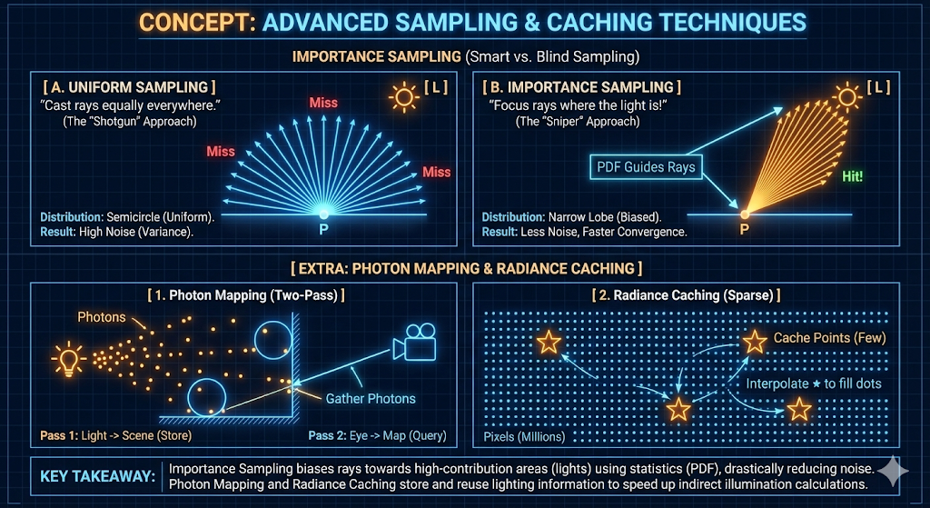
To address the stochastic nature of ray tracing, several techniques are employed to reduce noise and accelerate convergence without increasing the sample count prohibitively.

• Importance Sampling: rather than casting rays uniformly in all directions, ray directions are biased toward pathways that contribute most significantly to the final image, such as towards light sources or along specular reflection vectors. This statistical bias drastically increases the probability of sampling high-contribution areas, resulting in faster convergence and reduced variance (noise).
• Photon Mapping: This is a two-pass global illumination algorithm. The first pass (forward tracing) emits “photons” from light sources into the scene, storing them in a spatial map where they interact with surfaces. The second pass (backward tracing from the camera) queries this photon map to approximate indirect illumination efficiently.

• Radiance Caching: Because diffuse lighting changes slowly across surfaces, radiance values are computed at sparse locations and stored in a cache. Subsequent rays interpolate these cached values rather than performing expensive full-spectrum evaluations, exploiting the low-frequency nature of indirect lighting.

  

Low-Level CPU Optimization

Modern CPU architectures rely heavily on instruction pipelining. Efficient code must minimize pipeline stalls caused by unpredictable execution paths.

Branch Prediction and Branchless Programming

• The Problem (Branch Misprediction): CPUs utilize branch prediction to guess the outcome of conditional statements (if/else) and pre-load instructions into the pipeline. If the prediction fails (a “miss”), the pipeline must be flushed, causing a significant delay known as a Stall. In high-frequency loops like ray intersection, this penalty is severe.

• The Solution (Branchless Code): Conditional jumps should be replaced with arithmetic or bitwise operations wherever possible. For example, utilizing min() / max() functions or conditional moves allows the CPU to execute instructions linearly without risking pipeline flushes.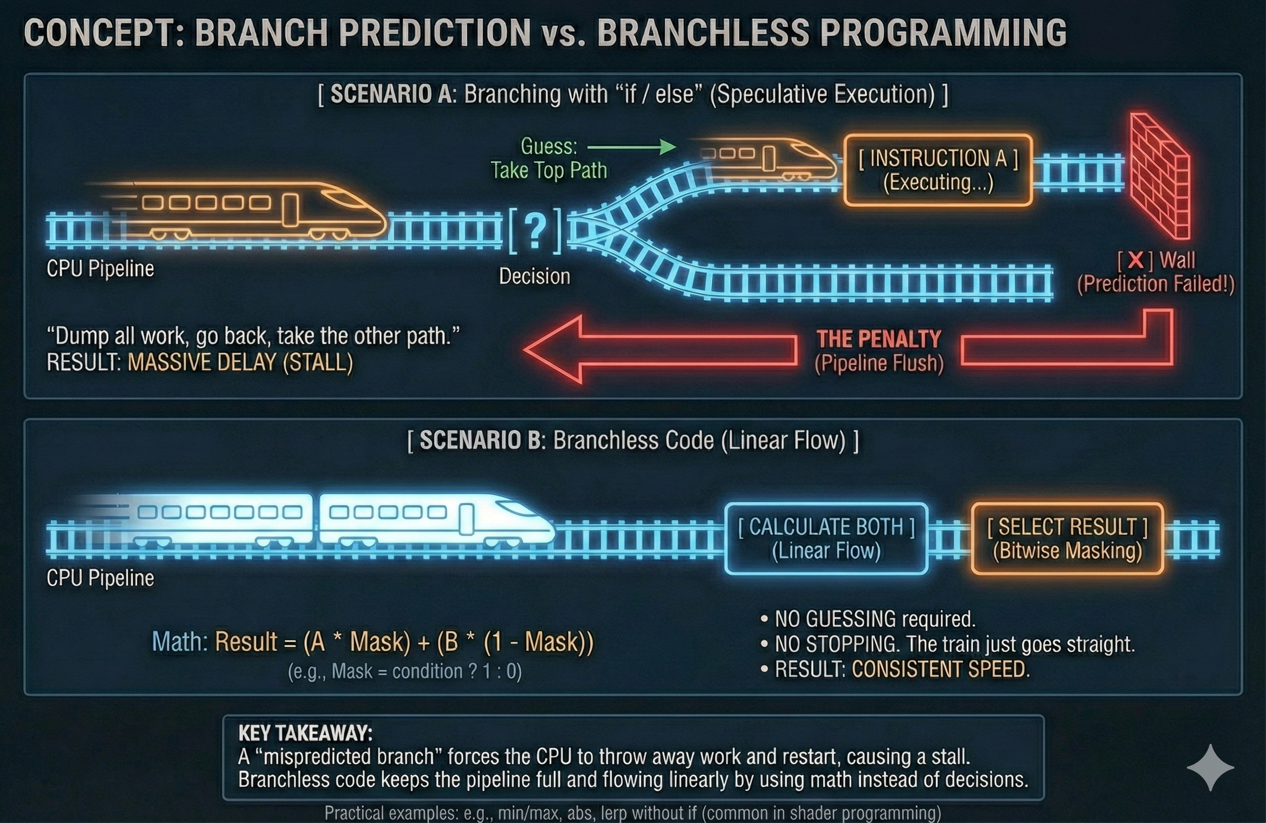

  

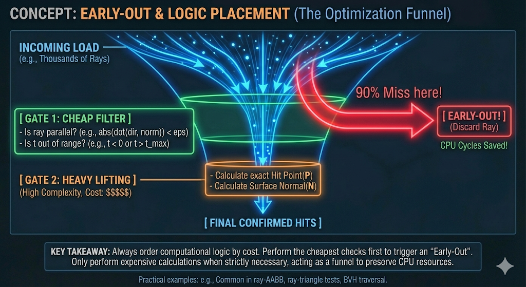
Early-Out and Logic Placement

• Complexity Management: Computational logic should be ordered by cost. The most inexpensive checks (lowest computational complexity) must be performed first to trigger an Early-Out.

• Application (Ray-AABB): Before calculating exact intersection points, simple checks—such as verifying if the ray is parallel to the slab ($D_x \approx 0$) or if the entry time exceeds the exit time ($t_{start} > t_{end}$)—are executed. This ensures that the expensive algebraic operations required for a precise hit are only performed when strictly necessary, preserving CPU cycles.

  

Instancing and Spatial Transformations

Instancing is a fundamental optimization that reuses a single mesh while applying unique transformations (SRT) to place objects in Global Space. The transformation is calculated using the column-vector convention, where the operation sequence is applied from right-to-left: Scaling $\rightarrow$ Rotation $\rightarrow$ Translation.

The Geometry of Transformation: Space Transformation

The concept of Space Transformation is fundamental to instancing and efficient scene management. It enables objects defined in their own Local Space to be correctly placed, oriented, and scaled within the global scene coordinates (Global Space).

Matrix Representation via Homogeneous Coordinates

• Transformations are practically executed using $4 \times 4$ matrices combined with Homogeneous Coordinates ($\mathbf{x, y, z, w}$).
  • The ‘w’ Coordinate:
    • $w=1$: The vector represents a position and is affected by translation.
    • $w=0$: The vector represents a direction and is unaffected by translation.
• The Transformation Matrix ($\mathbf{M}$) is a concise representation where its columns define the three basis axes and the origin of the new space:

\[\mathbf{M} = \begin{pmatrix} \vec{a}_x & \vec{b}_x & \vec{c}_x & O_x \\ \vec{a}_y & \vec{b}_y & \vec{c}_y & O_y \\ \vec{a}_z & \vec{b}_z & \vec{c}_z & O_z \\ 0 & 0 & 0 & 1 \end{pmatrix}\]

Hierarchical Space Transformation

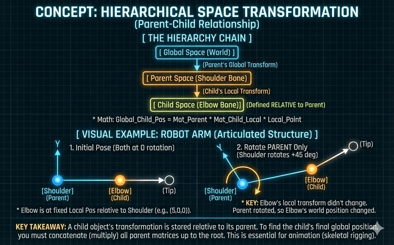
• Complex scenes and models use a Hierarchy of connected spaces (e.g., Global $\rightarrow$ Parent $\rightarrow$ Child) for efficient management.
  • Core Principle: An object’s Local Transformation is applied relative to its parent’s coordinate system. The Global position is found by concatenating (multiplying in sequence) the transformation matrices of all ancestor spaces, from the local space up to the root space.
  • Application in Animation: This hierarchical principle is crucial for skinning and rigging. Animation data stores only local transformations for each Bone relative to its parent, ensuring high efficiency. The final World Matrix is calculated by recursively multiplying these local matrices up the bone chain, which is heavily optimized using the GPU.

  

The Transformation Pipeline (SRT)

• The final Model Matrix ($M_{model}$) is constructed as the product:

\[M_{model} = \mathbf{T} \cdot \mathbf{R} \cdot \mathbf{S}\]

• The transformation sequence is applied to a point vector $\mathbf{v}$ as $\mathbf{v}’ = M_{model} \mathbf{v}$.

  

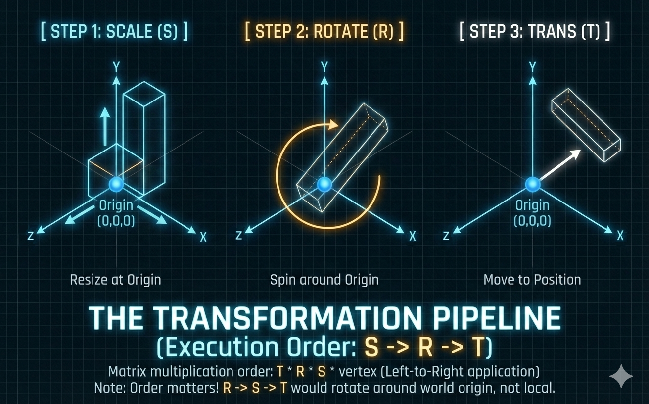
Scaling ($\mathbf{S}$)

• This is the first operation applied. It stretches or shrinks the object along its local axes using a diagonal matrix (presented here for 3D homogeneous coordinates).

\[\mathbf{S} = \begin{pmatrix} S_x & 0 & 0 & 0 \\ 0 & S_y & 0 & 0 \\ 0 & 0 & S_z & 0 \\ 0 & 0 & 0 & 1 \end{pmatrix}\]

• Note on Mirroring: Applying a negative scale (e.g., -1 on the X-axis) mirrors the object across the YZ plane. This reverses the winding order of vertices, which may require flipping surface normals to maintain correct lighting calculations.

Rotation ($\mathbf{R}$)

• This is the second operation applied. It defines the orientation of the object. For a rotation of $\theta$ around the Z-axis:

\[\mathbf{R}_z(\theta) = \begin{pmatrix} \cos\theta & -\sin\theta & 0 & 0 \\ \sin\theta & \cos\theta & 0 & 0 \\ 0 & 0 & 1 & 0 \\ 0 & 0 & 0 & 1 \end{pmatrix}\]

• For inverse rotation ($-\theta$), the properties of trigonometric functions ($\sin(-\theta) = -\sin\theta$, $\cos(-\theta) = \cos\theta$) are used, resulting in the transpose of the rotation matrix (since rotation matrices are orthogonal).

Translation ($\mathbf{T}$)

• This is the final operation applied. It shifts the local space origin $(0,0,0)$ to the new global position $(T_x, T_y, T_z)$.

\[\mathbf{T} = \begin{pmatrix} 1 & 0 & 0 & T_x \\ 0 & 1 & 0 & T_y \\ 0 & 0 & 1 & T_z \\ 0 & 0 & 0 & 1 \end{pmatrix}\]

Derivation of the Rotation Matrix

• The $2\times2$ rotation matrix for rotation around the Z-axis by an angle $\theta$ is derived by observing how the basis vectors $\hat{\mathbf{x}} = (1, 0)$ and $\hat{\mathbf{y}} = (0, 1)$ transform.

Transforming the X-axis Basis Vector

• The unit vector on the X-axis, $P_x = (1, 0)$, when rotated by $\theta$, moves to a new position $P_{x’}$:

  \[P_{x'} = (\cos\theta, \sin\theta)\]

• This vector forms the first column of the rotation matrix.

Transforming the Y-axis Basis Vector

• The unit vector on the Y-axis, $P_y = (0, 1)$, when rotated by $\theta$, moves to:

  \[P_{y'} = (-\sin\theta, \cos\theta)\]

• This vector forms the second column of the rotation matrix.

Final Rotation Matrix

• Applying these two new basis vectors as the columns allows us to rotate any vector $(x, y)$:

\[\begin{pmatrix} x_{rot} \\ y_{rot} \\ 1 \end{pmatrix} = \begin{pmatrix} \cos\theta & -\sin\theta & 0 \\ \sin\theta & \cos\theta & 0 \\ 0 & 0 & 1 \end{pmatrix} \begin{pmatrix} x_{orig} \\ y_{orig} \\ 1 \end{pmatrix}\]

• The resulting coordinates are:

\[x_{rot} = \cos\theta \cdot x_{orig} - \sin\theta \cdot y_{orig}\] \[y_{rot} = \sin\theta \cdot x_{orig} + \cos\theta \cdot y_{orig}\]

Inverse Transformation and Performance

• The inverse of the model matrix is required to convert a point from Global Space back to Local Space:

\[M_{model}^{-1} = \mathbf{S}^{-1} \cdot \mathbf{R}^{-1} \cdot \mathbf{T}^{-1}\]

• The calculation of the full inverse matrix is computationally heavy.
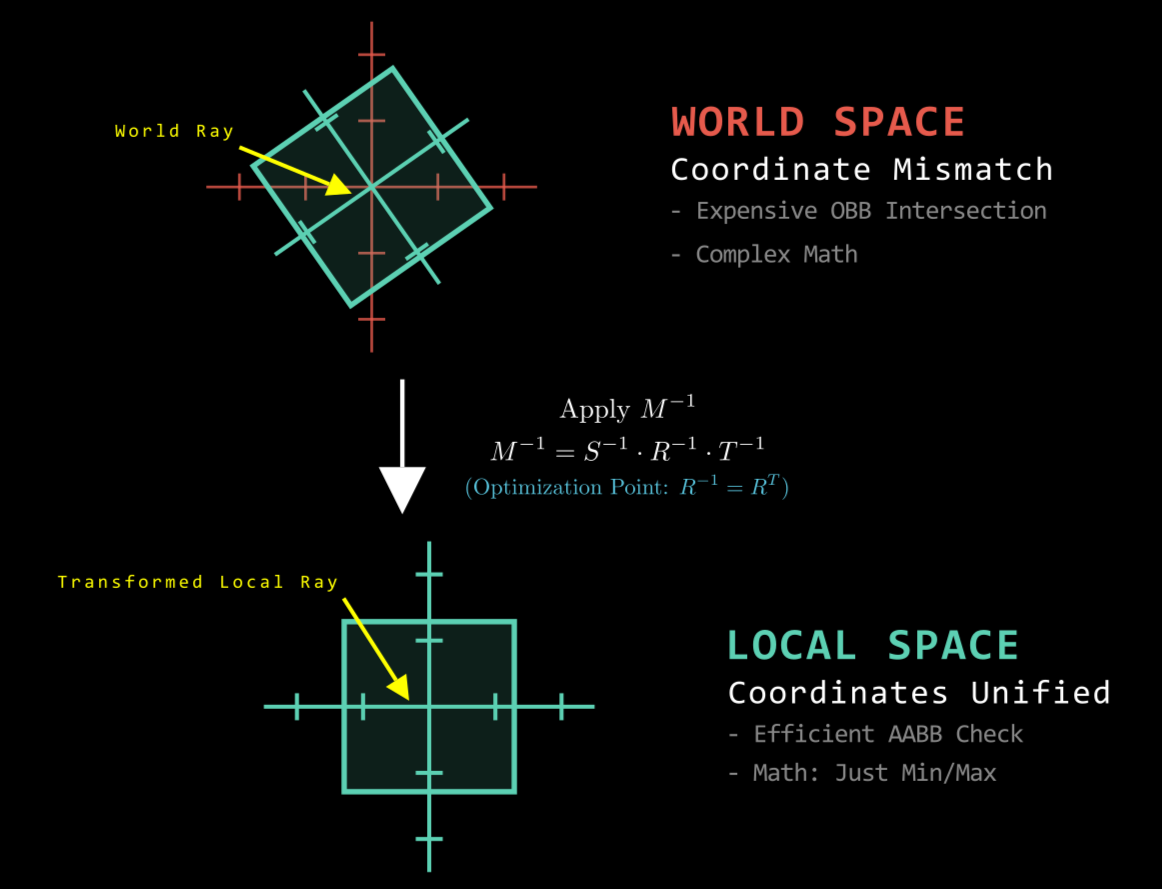
• However, the Rotation Matrix ($\mathbf{R}$) is an Orthogonal Matrix ($\mathbf{R}^{-1} = \mathbf{R}^{T}$).
  • This allows the inverse rotation component to be computed by a simple transpose operation, providing a significant performance gain when transforming rays or vectors into an object’s local space.

Optimization: The Inverse Ray Method

• A naive approach to collision detection for rotated instances involves rotating the AABB, which loosens the bounds and reduces efficiency. A superior approach is to transform the Ray into the Object’s Local Space.

• Concept: instead of checking “Ray vs. Rotated Box” in World Space, the engine checks “Inverse-Transformed Ray vs. Axis-Aligned Box” in Local Space.

• Implementation: The ray $R(t) = Q + t\vec{d}$ is transformed using the inverse model matrix ($S^{-1} \cdot R^{-1} \cdot T^{-1}$). In Local Space, the object is always axis-aligned, allowing for the use of highly optimized AABB intersection algorithms rather than complex OBB (Oriented Bounding Box) tests.

  

Extended Note: The Connection to AI/Machine Learning

• The fundamental principle of Space Transformation extends directly to core operations in AI/Machine Learning.
• AI layers consist primarily of matrix multiplications, which can be viewed as applying a continuous series of space transformations to the input data.
• Machine learning is the iterative process of adjusting the elements (weights) within these transformation matrices to map the input data space to a final, desired output space (the prediction).

Bounding Volume Hierarchy (BVH) Comprehensive Review

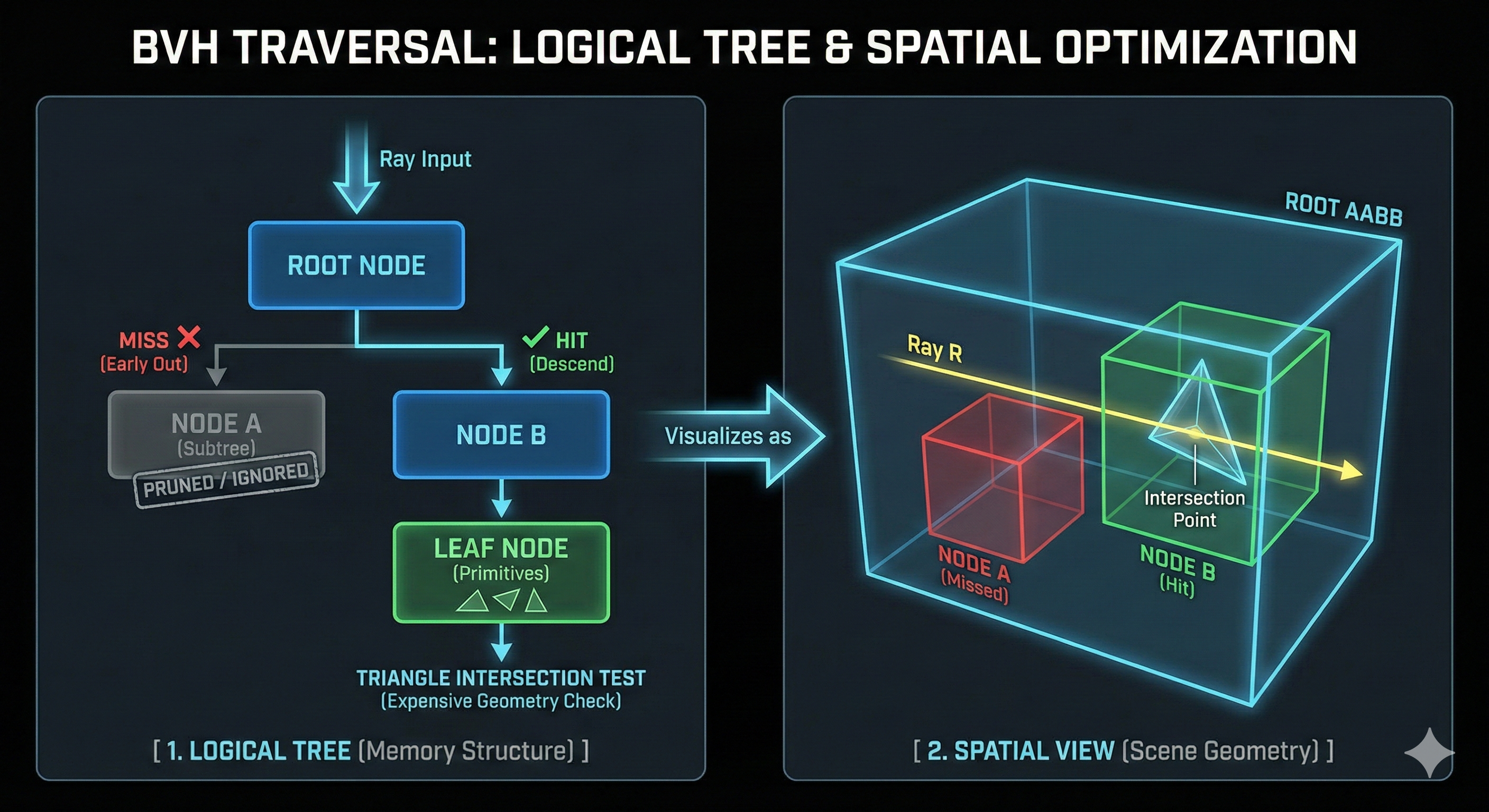
The Bounding Volume Hierarchy (BVH) is a core spatial partitioning data structure used to enable computationally intensive tasks such as real-time ray tracing. The primary goal of BVH is to dramatically reduce the number of ray-primitive intersection tests, thereby lowering the computational complexity from $O(M)$ (linear search) to $O(\log M)$ (logarithmic search).

Core Concept and Operating Principle

• The fundamental idea of BVH stems from an optimization mindset: replacing thousands of complex geometric tests with a minimum number of fast volume checks.

Basic Structure: Rapid Rejection

• Primitive Enclosure: Instead of performing a ray test against every single triangle or object ($M$ primitives), groups of objects are enclosed by a simple container called a bounding volume (typically an Axis-Aligned Bounding Box, AABB).
• Early Rejection: Checking if a ray intersects an AABB only requires a few simple arithmetic comparisons. If a ray misses the AABB, it is guaranteed to miss all the complex geometry contained within. This allows an immediate Early-Out of a large group of geometry with one single, fast test.

Hierarchical Structure and Two-Stage Traversal

Since a single bounding box cannot handle a complex scene, these volumes are organized into a hierarchical structure, usually in the form of a binary tree.

• High-Level Traversal: The ray traverses the BVH starting from the root node. The bounding box of each node is checked first, and if missed, the entire subtree is safely discarded.

• Low-Level Check: Only when the ray reaches a leaf node (containing a small number of primitives, typically 1 to 4) is the costly intersection test against the actual geometry performed.

  

BVH Construction and Optimization

• The performance gain of a BVH is heavily dependent on how the structure is built.

Construction Algorithm and SAH

• Partitioning Method: The common high-quality construction method is top-down partitioning. It starts with a single volume encompassing all objects and recursively divides it into smaller volumes.
• Splitting Criterion: For efficient traversal, objects are sorted along the longest axis of the current bounding box. Splitting is then performed based on a criterion, often half the count of objects.
  • Reason for Sorting: Sorting allows for efficient spatial management, and splitting along the longest axis minimizes the surface area of the resulting child nodes.
• Surface Area and Optimization: The probability of a ray hitting a volume is proportional to that volume’s surface area. Minimizing the surface area reduces the possibility of unnecessary intersection tests, accelerating optimization.
• Surface Area Heuristic (SAH): The most effective split is chosen by minimizing the sum of the total surface areas of the child volumes. This is the industry-standard method for minimizing the average ray traversal cost.

Dynamic Scene Optimization: Temporal Coherence

In dynamic environments where objects in the scene are moving, the cost of completely rebuilding the BVH every frame must be mitigated.

• Leveraging Temporal Coherence: This technique exploits the fact that the movement of objects between consecutive frames is usually small.
• Implementation: The BVH from the previous frame is either reused or quickly updated/refitted. This is significantly faster than rebuilding from scratch, improving the overall frame rate, and is a core mindset of “frame-level optimization.”

Deep Dive into Implementation: AABB Intersection Test (Slab Method)

• The AABB intersection test is the core of BVH traversal, and the Slab method is used alongside branchless code implementation for high performance.

Slab Method and $t_{enter}, t_{exit}$ Calculation

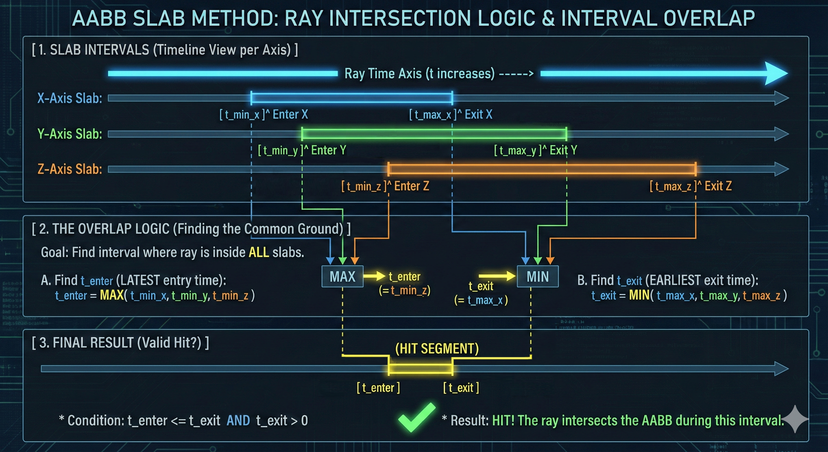
• Slab Definition: The AABB is regarded as the intersection of three pairs of parallel planes (Slabs).

• Time Calculation: For each axis ($x, y, z$), the parameter time $t$ at which the ray enters ($t_{min}$) and exits ($t_{max}$) the corresponding Slab is calculated from the ray equation:

  \[t_{slab} = \frac{p_{plane} - Q_{origin}}{d_{axis}}\]
• Branchless Code: Since the $t$ values are relative to the ray’s direction, $\min() / \max()$ functions are used to determine $t_{min}$ and $t_{max}$. This is a key optimization that eliminates conditional statements (if) and prevents performance degradation (Stall) due to CPU’s Branch Misprediction.

• Final Intersection Check: The intersection of the time intervals for all three axes is found:

  \[t_{enter} = \max(t_{min\_x}, t_{min\_y}, t_{min\_z})\] \[t_{exit} = \min(t_{max\_x}, t_{max\_y}, t_{max\_z})\]

  The intersection is valid when $t_{enter} \le t_{exit}$.

• Validity Check: The intersection time must satisfy $t_{enter} > 0$. For numerical stability, only $t_{enter} > \mathbf{\epsilon}$ (epsilon) is considered a valid intersection. (If $t_{enter} < 0$, the AABB is behind the ray origin and is invalid.)

  

Zero Division Handling and Reciprocal Optimization

Handling the situation where the denominator is zero (the ray is parallel to an axis) is essential for the robustness and performance of the intersection test.

• Reciprocal Use: Multiplication is faster than division on the CPU, so the reciprocal of the ray direction vector ($1/d_{axis}$) is pre-calculated to replace division with multiplication.
• Handling $d_{axis} = 0$: If $d_{axis}$ was 0, its reciprocal is treated as a pre-defined infinity or a very large value. The sign of infinity is determined by the sign of the numerator ($p_{plane} - Q_{origin}$).
  • Parallel and Miss: If only the denominator is zero and the ray is outside the Slab, no intersection will ever occur, and an immediate Early-Out is performed.
  • Parallel and On Plane: If the ray origin is exactly on the plane (form $0/0$), NaN may occur numerically. This is handled by methods such as extending the AABB boundaries by $\epsilon$, and it is usually considered non-intersecting to ensure stability.

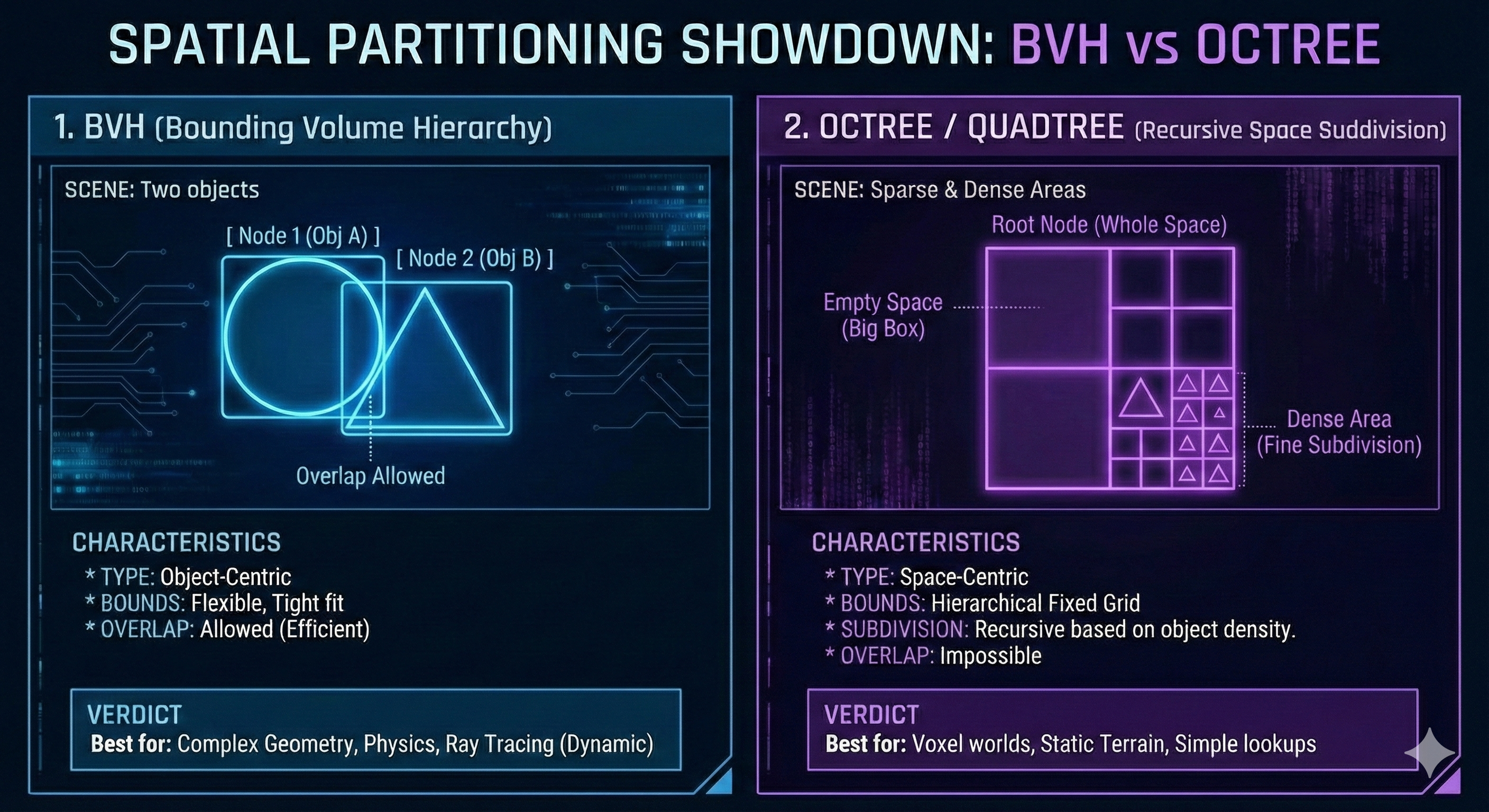
BVH vs. Octree: Differences in Spatial Partitioning

Feature	Bounding Volume Hierarchy (BVH)	Octree / Quadtree
Core Concept	Primitive Partitioning: Object-centric	Space Partitioning: Space volume-centric
Partitioning Method	Flexible binary split based on object count and SAH	Fixed split of space into 8 (3D) equal-sized volumes
Child Node Overlap	Overlap between child bounding volumes is allowed.	No overlap between partitions (mutually exclusive).
Physics/Collision Application	Child volume overlap is allowed, avoiding the object duplication problem. Preferred in physics engines.	Object duplication or special handling is required if objects straddle boundaries.

Because BVH volumes are flexibly formed according to the distribution of geometry, they are significantly more efficient than the fixed grid partitioning of an Octree in complex and non-uniformly distributed scenes.

Floating-Point Encoding

Core Concept

• Floating-Point Encoding is a standardized method used by computers to represent a vast range of real numbers—from extremely small fractions to very large magnitudes—within a limited number of bits. T
• his representation is fundamentally composed of three fields:
  1. Sign: Determines whether the number is positive or negative.
  2. Mantissa (or Significand): Stores the significant digits or precision of the number.
  3. Exponent: Stores the power of the base (usually 2) that the mantissa is multiplied by.

  

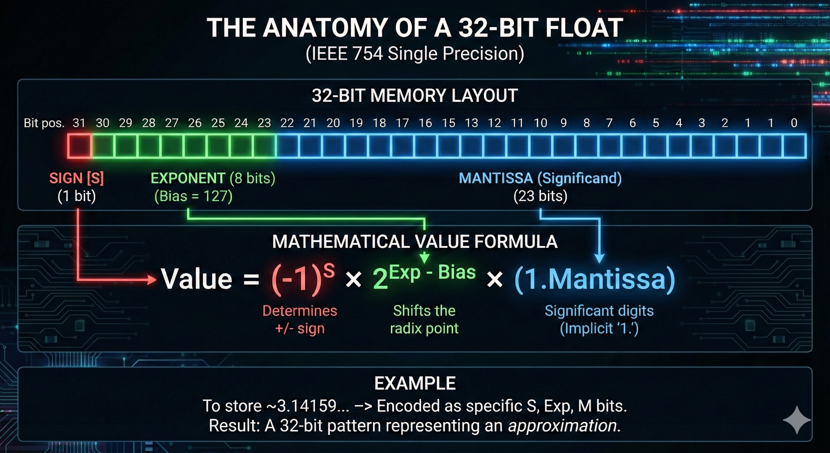
The Role of the Exponent

• The floating-point system uses the exponent to effectively shift the position of the radix point in the binary number.
  • This shift dramatically expands the range of values that can be represented.
• Example: The binary number $110.11_2$ is normalized into scientific notation as $1.1011_2 \times 2^{+2}$. In this case, the exponent is $+2$.
• Significance: This mechanism allows a machine using a fixed number of bits (e.g., 32-bit single precision) to cover a range far greater than what fixed-point or integer formats can achieve, albeit at the cost of precision.

Fundamental Challenge

• In computer graphics, Floating-Point Encoding is employed to represent a wide spectrum of numbers, from minuscule fractions to immense values, using a constrained number of bits.
  • This is crucial for tasks like storing High Dynamic Range (HDR) color data , where luminance values often exceed 1.0.
• The Problem of Approximation:
  • This encoding method inherently relies on approximations.
  • Consequently, it is challenging to accurately represent the exact real number zero or to reliably compare two floating-point values for exact equality.
  • This fundamental limitation introduces numerical stability issues.

Resolution Strategy

• These precision limitations can lead to unwanted artifacts or logical failures throughout the rendering pipeline, particularly in high-precision operations such as ray intersection testing and depth comparisons.
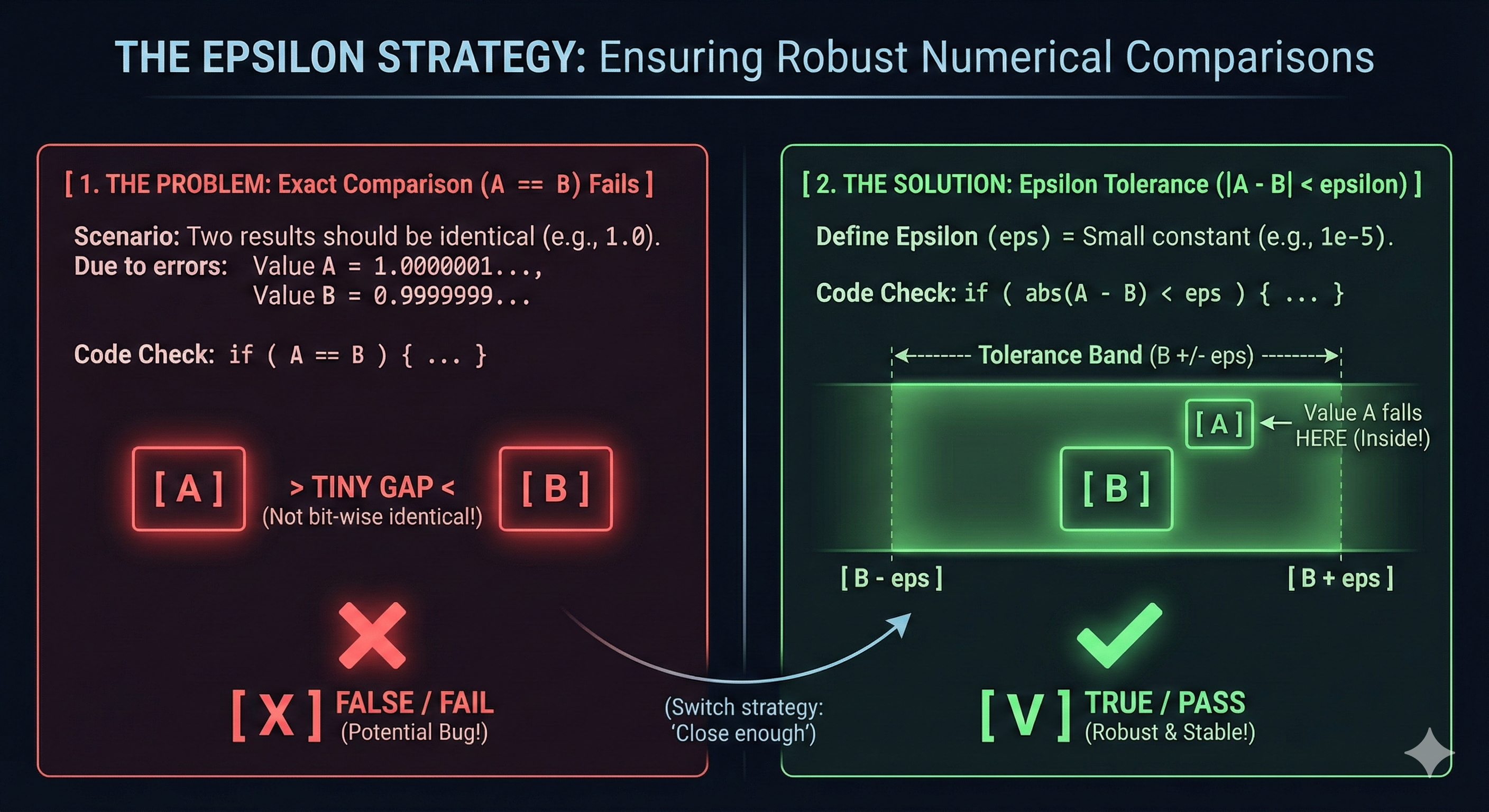
• The primary strategy for ensuring numerical stability and achieving robust rendering optimization is the use of the Epsilon ($\mathbf{\epsilon}$) Offset.
  • $\mathbf{\epsilon}$ is defined as a very small, positive constant (e.g., $10^{-4}$ or $10^{-6}$).
• Instead of checking for exact equality ($\mathbf{A == B}$),
  • algorithms check if the two values are “sufficiently close” or if “one value is marginally greater than the other”.
• Conditional Check:
  • When comparing $\mathbf{A}$ and $\mathbf{B}$, a condition like $\mathbf{A > B + \epsilon}$ is used.
  • This deliberately permits a minute precision error, ensuring the comparison is robust against floating-point inaccuracies.

• This systematic application of the Epsilon offset is an essential technique for achieving the necessary reliability and performance in modern computer graphics.

  

Top