3D Physics Engine

한국어

Custom 3D Physics Engine

1. Project Overview

• This project demonstrates the development of a comprehensive 3D Physics Engine implemented in C++ using Win32 API and DirectX 12.
• The primary objective was to engineer a physics simulation from scratch, devoid of commercial middleware, to gain a deep understanding of rigid body dynamics, collision detection pipelines, and constraint resolution strategies common in modern game development.
• The engine features a robust Hybrid Collision Resolution system, an optimized Sweep and Prune (SAP) broad-phase, and a powerful Visual Debugging Suite designed to validate complex physical interactions.

Core Tech Stack

• Language: C++ (Modern C++17 Standards)
• Graphics/System: DirectX 12, Win32 API
• Key Algorithms: Sweep and Prune (SAP), GJK, EPA, Sequential Impulse Solver, Continuous Collision Detection (CCD).

2. Architecture & Pipeline

• The simulation executes a multi-stage pipeline designed to balance performance and accuracy:

1. Integration

• Updates linear and angular velocities along with positions based on accumulated forces, including gravity, external impulses, and user intervention.

2. Broad Phase

• Rapidly culls non-colliding pairs using axis-sorting algorithms (Sweep and Prune) to minimize the computational workload for subsequent stages.

3. Narrow Phase

• Precisely determines collision manifolds, including contact points and normals, utilizing Convex Hull algorithms (GJK/EPA) for accurate intersection testing.

4. Resolution

• Solves mechanical constraints and contact penetrations using a sequential impulse-based solver to ensure physical stability.

3. Collision Detection

3.1. Broad Phase: Optimized Sweep and Prune (SAP)

• To efficiently manage scenes with high object counts, the engine utilizes the Sweep and Prune (SAP) algorithm.
• A significant optimization implemented here is Dynamic Axis Selection.
  • Instead of adhering to a fixed axis, the system evaluates the spatial variance of objects each frame and sorts them along the axis with the largest extent.
  • This minimizes the number of overlapping intervals on the projection axis, significantly reducing false positives.
• Implementation Highlight:
  • The implementation ensures memory safety and avoids $O(N^2)$ checks by maintaining an active list of overlapping bodies.

    void SweepAndPrune1D(const Body* bodies, const int numBodies, std::vector<collisionPair_t>& finalPairs, const float deltaSecond) {
        // Optimization: Use std::vector to prevent stack overflow in dense scenes
        std::vector<pseudoBody_t> sortedBodies(numBodies * 2);
  
        // 1. Calculate Bounds & Select Optimal Axis
        SortBodiesBounds(bodies, numBodies, sortedBodies.data(), deltaSecond);
  
        // 2. Build Collision Pairs using Active List approach (O(N + K))
        BuildPairs(finalPairs, sortedBodies.data(), numBodies);
    }
  
    void BuildPairs(std::vector<collisionPair_t>& collisionPairs, const pseudoBody_t* sortedBodies, const int numBodies) {
        // Note: finalPairs is cleared in the caller (BroadPhase)
        std::vector<int> activeList; // Stores IDs of currently overlapping bodies
  
        const int doubleNumBodies = numBodies * 2;
        for (int i = 0; i < doubleNumBodies; ++i) {
            const pseudoBody_t& targetBody = sortedBodies[i];
            int bodyId = targetBody.id;
  
            if (targetBody.isMin) {
                // Body enters the sweep axis: Pair with all currently active bodies
                for (int activeId : activeList) {
                    collisionPair_t pair;
                    pair.a = std::min(bodyId, activeId);
                    pair.b = std::max(bodyId, activeId);
                    collisionPairs.push_back(pair);
                }
                activeList.push_back(bodyId);
            } else {
                // Body exits the sweep axis: Remove from active list
                auto it = std::remove_if(activeList.begin(), activeList.end(),
                    [bodyId](int id) { return id == bodyId; });
                activeList.erase(it, activeList.end());
            }
        }
    }
  

3.2. Narrow Phase: GJK & EPA

• For precise collision detection between convex polyhedra, the engine employs the Gilbert-Johnson-Keerthi (GJK) algorithm.
• Intersection Test:
  • GJK iteratively constructs a simplex inside the Configuration Space Object (CSO) to determine if it encloses the origin.
• Contact Generation:
  • Upon collision, the Expanding Polytope Algorithm (EPA) is triggered to calculate the penetration depth and contact normal by expanding the simplex to the CSO boundary.
• For performance-critical primitives like spheres, specialized algebraic tests (Ray-Sphere, Sphere-Sphere) are implemented to bypass expensive GJK iterations.

4. Hybrid Collision Resolution

• The engine intelligently dispatches detected contacts to different solvers based on the collision context.

4.1. Continuous Collision Detection (CCD)

• To mitigate the “tunneling effect” where high-velocity objects pass through geometry, a Predictive Impulse Solver is implemented.
• Mechanism:
  • The system calculates the Time of Impact (TOI) for dynamic objects.
• Execution:
  • Contacts are sorted by TOI.
  • The simulation advances to the earliest impact time ($TOI > 0$), resolves the collision, and repeats.
  • This guarantees that fast-moving objects interact correctly with static environments.

4.2. Sequential Impulse Solver

• For static contacts ($TOI = 0$) and mechanical constraints (joints, resting contact), an Iterative Constraint Solver is utilized.
• This solver applies “Warm Starting”—using the previous frame’s solution as an initial guess—to ensure stability in complex stacking scenarios.

5. Visual Debugging Suite

• A significant focus of this project was the development of Runtime Inspection Tools, acknowledging that rigorous visual validation is critical for physics programming.

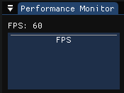
5.1. Performance Monitor

• A real-time performance graph tracks the current FPS and CPU load.
• This provides immediate feedback on the efficiency of optimization techniques during stress testing.

5.2. Interactive Object Inspector

• Users can pause the simulation and select objects via mouse picking.

  Property Inspector

• The inspector panel reveals real-time physical properties, including Linear/Angular Velocity, Mass, and Orientation.

Gizmo Manipulation

• Selected objects can be translated or rotated using a 3D gizmo.
• The physics state is automatically managed (velocity reset) to ensure stability after manipulation.

5.3. Deep Contact Visualization

• To verify the accuracy of the Narrow Phase and Solver, the engine offers detailed visualization modes:

Collision Metadata Visualization

• Wireframe Rendering Mode:
  • To mitigate visual occlusion during overlap, the system supports a wireframe rendering mode for active entities and their associated collision pairs.
  • This ensures the internal state of the simulation remains visible.

  

• Manifold & Primitive Identification:
  • Contact Data: Discrete contact points are rendered as red cubic markers, while the resulting collision normals are projected as yellow vectors, facilitating the empirical verification of the mathematical resolution.
  • Primitive Highlighting: For polyhedral shapes, the specific geometric primitive (triangle) identified by the narrow-phase algorithm is highlighted in blue, isolating the exact surface contributing to the contact manifold.

  

Hit Result Tree UI

• When multiple collisions occur, a tree view UI organizes all contact pairs, allowing developers to isolate and inspect specific manifolds.
• Selecting a specific contact point automatically highlights the corresponding subtree within the hierarchy.

5.4. Frame-by-Frame History (Rewind/Replay)

• Circular State Buffer:
  • To facilitate the analysis of high-speed collision events, a Circular History Buffer was implemented to cache the authoritative simulation state (Transform, Velocity) for the trailing 120 frames.
• Detached Execution:
  • Active Physics Stepping:
    • The engine supports active physics simulation starting from any restored historical frame.
    • This allows developers to test collision resolution logic in a paused environment without affecting the main game loop.
  • State Restoration:
    • Any simulation steps performed during this rewind phase are treated as speculative data.
    • Upon resuming the live session, the engine discards these changes and reloads the latest cached state, ensuring the continuity of the original gameplay timeline.

  

6. Stress Test & Validation

• A dedicated stress test scene was created to benchmark the engine’s performance and stability under various conditions.

6.1. Test Environment Setup

• The scene offers configurable parameters to test different subsystems:
• Density (Dense vs. Sparse): Controls object spacing.
  • Dense: Objects are tightly packed to rigorously test SAP overlap checks.

  

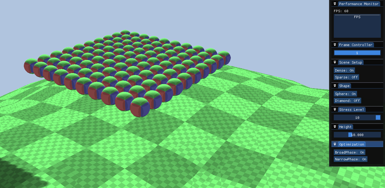
  • Sparse: Objects are spread out to verify culling efficiency.

  

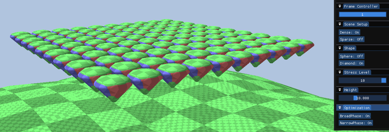
• Shape Selection:
  • Sphere: Tests analytic collision algorithms.
  • Diamond (Convex): Tests the performance of GJK/EPA algorithms.

  

• Initial Height:
  • The initial height can be modified to adjust the potential energy to test high-impact stability and stacking behavior.

  

6.2. Optimization Verification

• A runtime toggle for the Broadphase Optimization allows for immediate A/B testing between the Sweep and Prune (SAP) algorithm and a brute-force baseline.
• This setup validates the algorithm’s efficiency across different spatial distributions.

Dense Scenario

• In the Dense configuration, objects are tightly clustered, resulting in a high degree of spatial overlap.

• Analysis:
  • As observed in the figures above, the performance delta is minimal in the dense scenario.
  • Due to the high concentration of objects, the number of potential collision pairs remains high regardless of the broadphase strategy.
  • Consequently, the SAP algorithm cannot effectively cull pairs, shifting the computational load primarily to the Narrowphase.

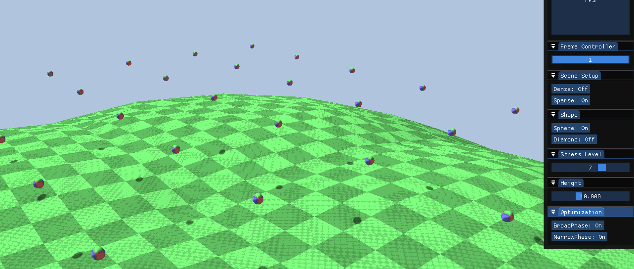
Sparse Scenario

• In the Sparse configuration, objects are widely distributed across the scene.

• Analysis:
  • The performance gap becomes distinct in this scenario.
  • The SAP algorithm effectively prunes distant, non-interacting objects, maintaining a stable framerate.
  • In contrast, the brute-force approach suffers from significant performance degradation due to its complexity, wasting cycles checking collisions between objects that are far apart.

7. Sandbox Scene

• The Sandbox scene serves as a comprehensive validation environment, showcasing typical simulation scenarios to verify the stability and versatility of the constraint solver.

7.1. Simulation Scenarios

Stacked Boxes

• This validates the iterative solver’s convergence and stability.
• It specifically tests the effectiveness of “Warm Starting” in preventing jitter during vertical stacking.

Chain

• It tests Distance Constraints and error correction.
• This scenario verifies that links remain connected without stretching under gravity and tension.

Moving Platform

• This validates the interaction between Kinematic bodies (infinite mass) and Dynamic bodies.
• It tests friction application and relative velocity handling on moving surfaces.

Rotator

• It demonstrates Angular Velocity integration and collision response.
• This scenario tests how dynamic objects react to high-speed impacts from rotating kinematic obstacles.

Ragdoll

• This is a complex Articulated System test.
• It verifies hierarchical transformations and the stability of multiple constraints (joints and limits) working in unison.

8. Future Development

• To further enhance the engine’s capabilities and performance, the following improvements are planned:

Optimize Narrowphase

• Implement temporal coherence or more advanced caching for GJK to reduce computational overhead in persistent contacts.

Add More Cases in Sandbox

• Introduce complex compound shapes and additional constraint types (e.g., ball-and-socket, slider).

Add More Shapes in Stress Test

• Expand the test suite to include capsules and cylinders to validate a wider range of collision primitives.

Top