Computer Graphics: Camera
Camera
- This report outlines the fundamental principles of camera operation, both in the physical world and within the context of computer graphics.
- It covers concepts ranging from light convergence and focusing to the implementation of visual effects like defocus blur and anti-aliasing.
Constructing the Camera’s Basis Axes
- In 3D graphics, a camera’s local coordinate system is defined by three orthogonal basis vectors.
- These vectors are constructed to align with the camera’s orientation in the world, allowing for the correct projection of 3D objects onto a 2D viewport.
- The process relies on three key parameters:
- the camera’s position (lookfrom)
- the point it is aimed at (lookat)
- a world-space up vector
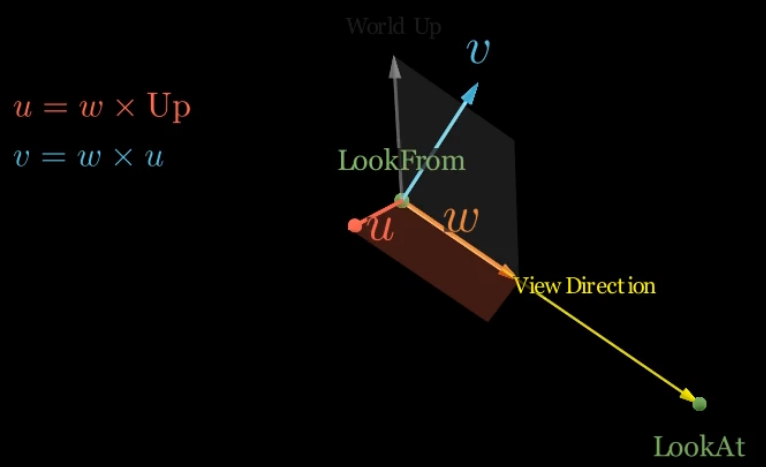
Defining the Camera’s Local Axes
- The camera’s local axes (typically referred to as the u-v-w basis or right-up-view basis) can be calculated using vector operations:
- View Direction (w-axis)
- The first axis is the camera’s view direction.
- This is a vector pointing from the
lookfromposition to thelookatpoint.
- This is a vector pointing from the
- To form a proper basis vector, it must be normalized.
- $w=\text{unit_vector}(\text{lookfrom}−\text{lookat})$
- The vector is defined as
lookfrom - lookatto ensure the w-axis points away from the scene, which is the standard convention for left-handed coordinate systems often used in computer graphics.
- The first axis is the camera’s view direction.
- Right Vector (u-axis)
- The second axis, or “right” vector, is perpendicular to both the view direction and the world-space up vector.
- It is computed using a cross product.
- The world-space up vector is typically $(0,1,0)$, but it’s important to use a normalized version of it in the calculation.
- $u=\text{unit_vector}(\text{up_vector}\times w)$
- The second axis, or “right” vector, is perpendicular to both the view direction and the world-space up vector.
- Corrected Up Vector (v-axis)
- The third axis is the “up” vector in the camera’s local space.
- It must be perfectly orthogonal to both the view direction and the right vector.
- While an initial up vector is provided, a new, corrected up vector is generated to ensure this orthogonality.
- This is also calculated using a cross product.
- $v=w\times u$
- The order of the vectors in the cross product is crucial for a right-handed or left-handed coordinate system.
- The order shown above is consistent with the left-handed system used in the initial derivation of $u$.
- The third axis is the “up” vector in the camera’s local space.
- View Direction (w-axis)
The Importance of Normalization
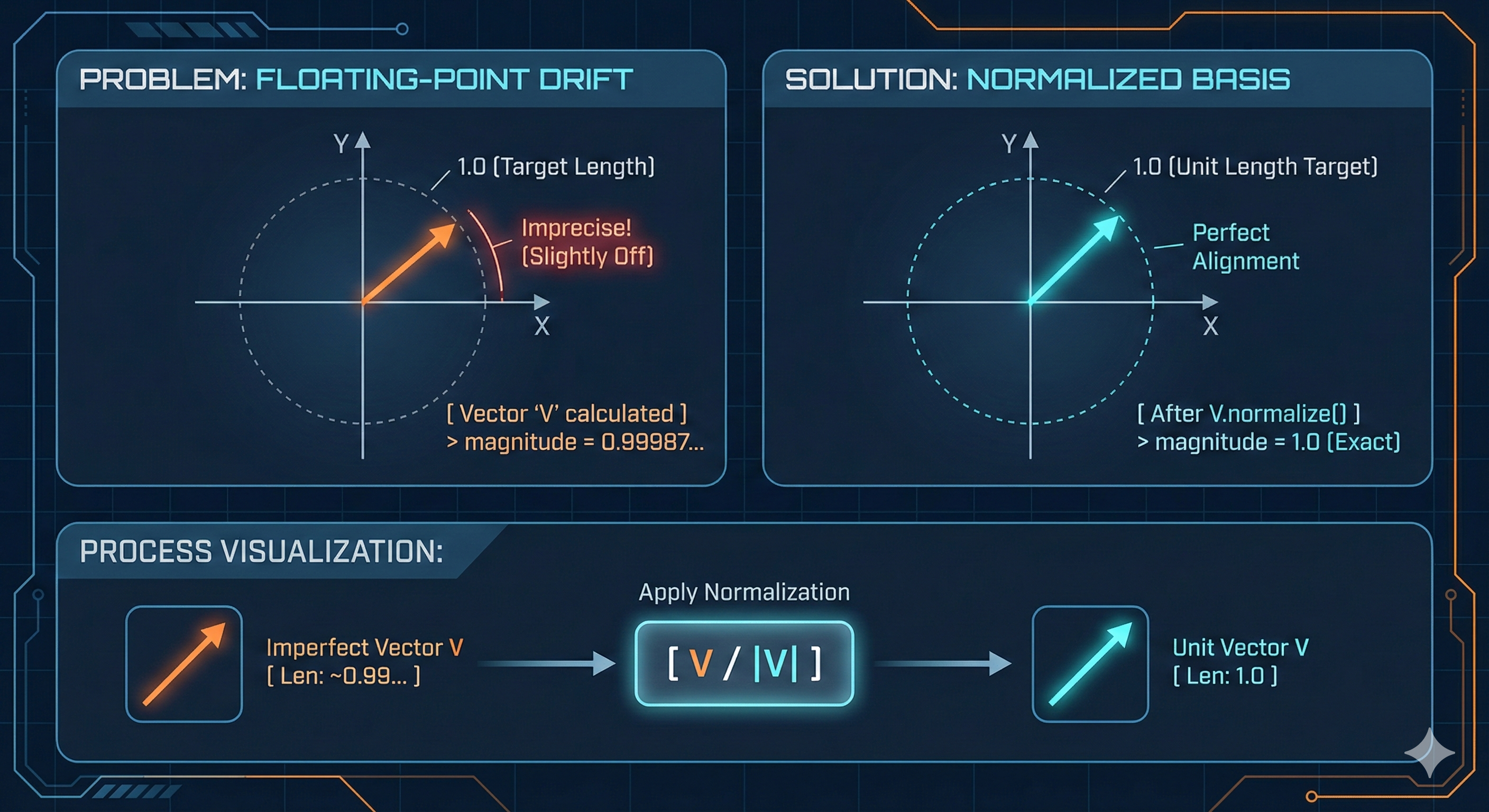
- While the cross product of two orthogonal unit vectors theoretically results in another unit vector, this isn’t always the case in practice.
- Due to the limitations of floating-point arithmetic, the computed magnitude may be slightly off from
1.
- Due to the limitations of floating-point arithmetic, the computed magnitude may be slightly off from
- Therefore, it is a standard and essential practice to normalize the resulting vectors after each cross-product operation.
- While the
lookfromandlookatpoints define a direction, the magnitude of the resulting vectors from subtraction and cross-product operations can vary. - Normalization ensures that each basis vector has a unit length, which is a fundamental requirement for a consistent and stable coordinate system.
- While the
-
This process is crucial for mitigating precision errors that can accumulate from repeated vector calculations.
How a Camera Forms an Image
Image Point and Image Plane
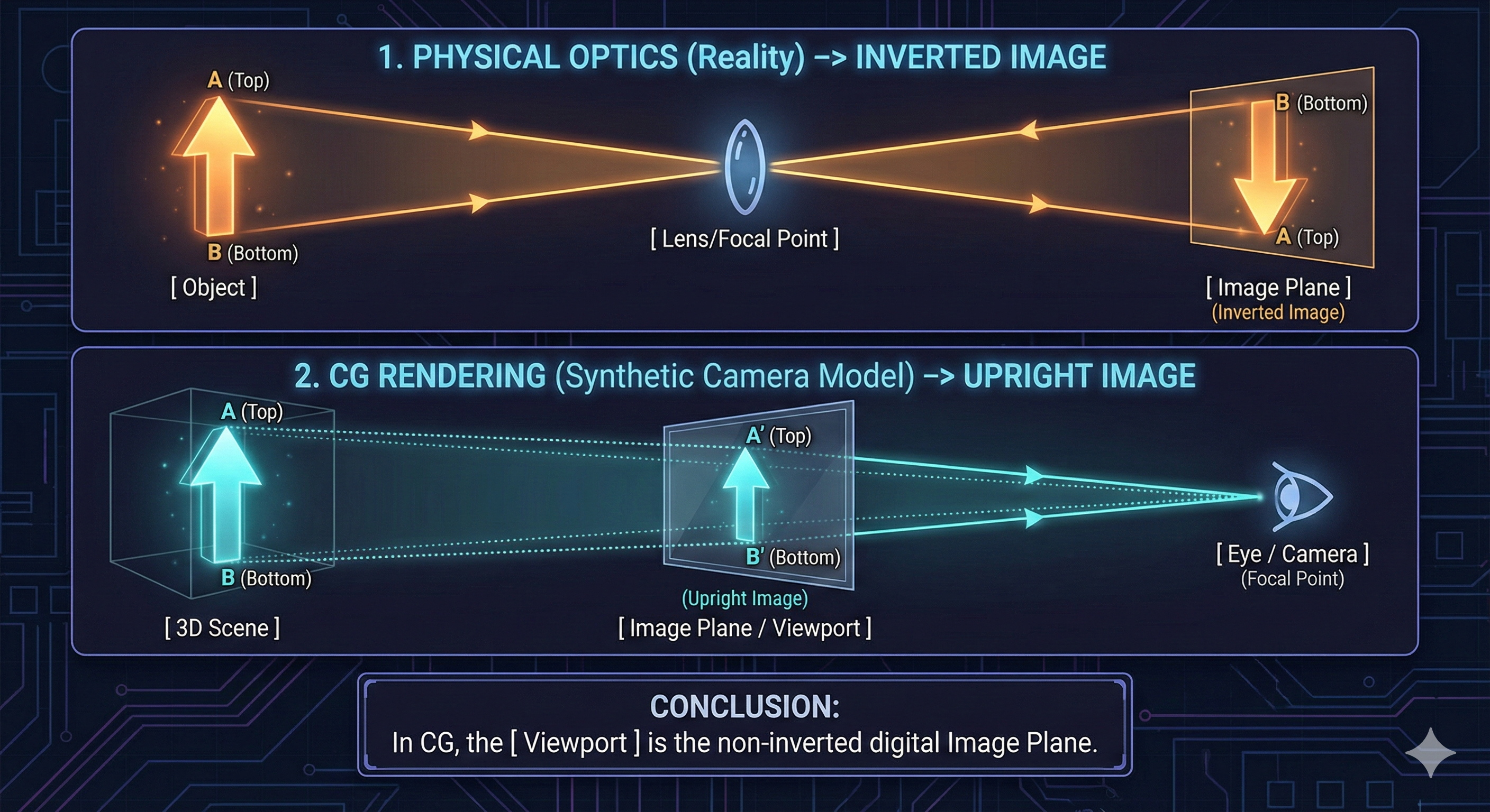
- A camera forms an image by converging light rays from an object onto a sensor.
- While an object reflects light in many directions, a camera’s lens focuses these rays to a single point, called the Image Point, on a 2D surface known as the Image Plane.
- Collectively, these points form an inverted image on the sensor.
- In computer graphics, the viewport is the 2D window on the screen where the 3D scene is rendered.
- It represents the final rendered image and can be considered the digital equivalent of the physical image plane.
Circle of Confusion (CoC)
- When light rays from a point on an object do not perfectly converge on the image plane, they form a small circle instead of a single point.
- This is known as the Circle of Confusion (CoC) .
- The size of the CoC directly determines an object’s sharpness in the final image.
- A smaller CoC results in a sharper, more in-focus image.
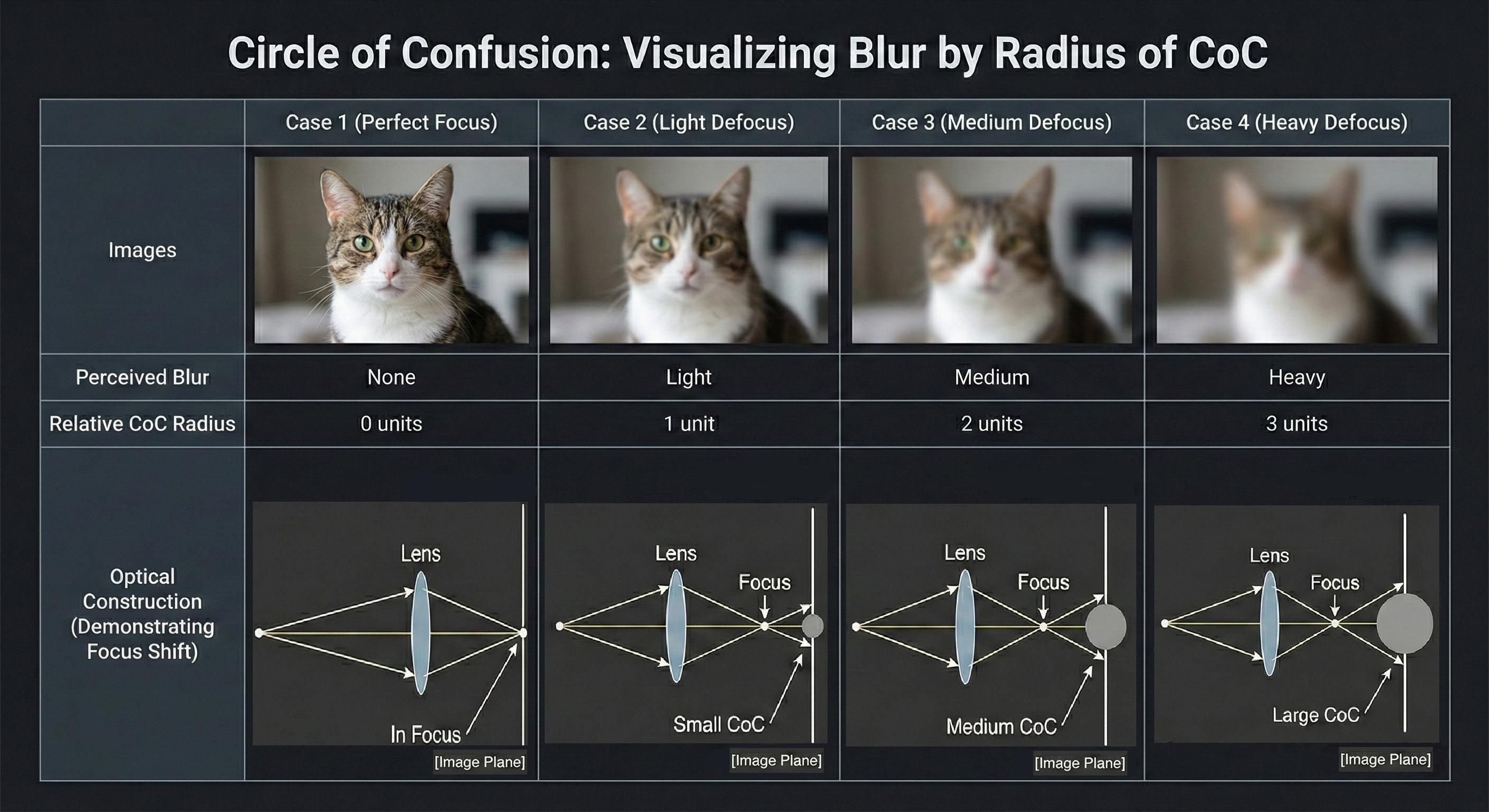
- By adjusting the lens, a photographer can control the size of the CoC for objects at different distances, thus bringing them into focus.
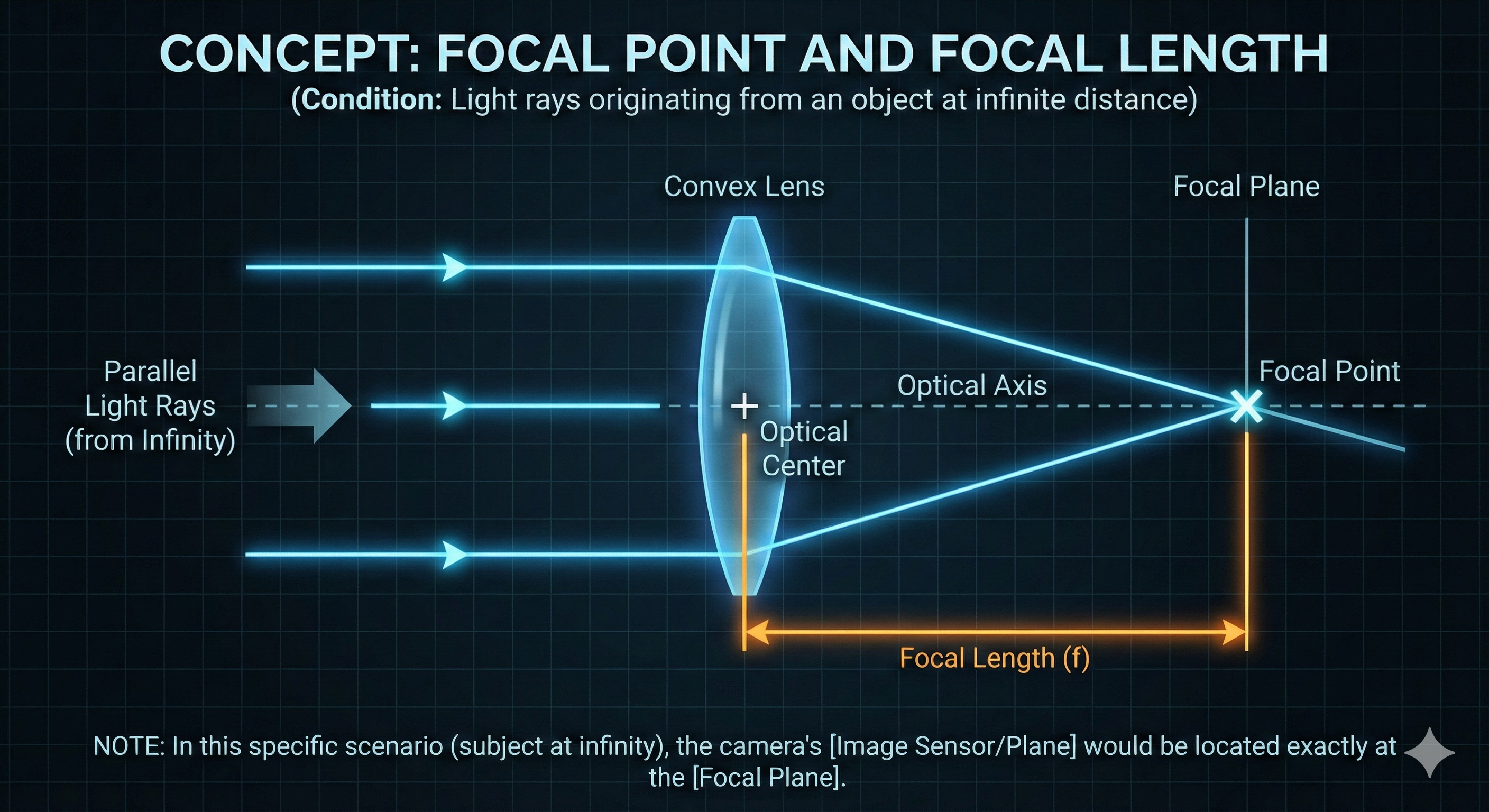
Focal Point and Focal Length
- The concepts of the Focal Point and Focal Plane are specific to light rays originating from objects at an infinite distance, where the rays are effectively parallel.
- In this scenario, all parallel rays converge to a single point on the Focal Plane, known as the Focal Point.
- Focal Length is the distance between a lens’s optical center and its principal focal point.
- For a real-world camera, if the subject is at an infinite distance, the image plane is at the same location as the focal plane,
- so the focal length can be considered the distance from the lens’s optical center to the image sensor.
- For a real-world camera, if the subject is at an infinite distance, the image plane is at the same location as the focal plane,
- Lenses are classified as either prime (fixed focal length) or zoom (variable focal length).
- A zoom lens changes its focal length by moving its internal elements, which alters the field of view.
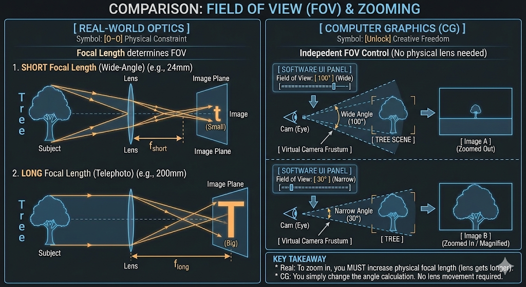
Field of View and Zooming
- The Field of View (FOV) is the extent of the observable world that is seen at any given moment.
- In photography and computer graphics, it is the angle that determines how much of a scene the camera can capture, essentially controlling the perspective and zoom level.
- In the real world, a camera’s field of view is intrinsically linked to the focal length.
- A specific lens with a fixed focal length (e.g., a 50mm lens) will have a specific, non-negotiable FOV.
- A longer focal length (telephoto lens) results in a narrower field of view, which magnifies the scene and produces a “zoomed-in” effect.
- Conversely, a shorter focal length (wide-angle lens) provides a wider field of view, capturing more of the scene and creating a “zoomed-out” effect.
- A specific lens with a fixed focal length (e.g., a 50mm lens) will have a specific, non-negotiable FOV.
- Unlike real-world cameras,
- computer graphics engines often allow the field of view to be set independently of the focal length for greater creative control, though this is not physically accurate.
Aperture
- In an optical system, the aperture is the opening that controls the amount of light entering the lens.
- A larger aperture permits light to enter from a wider range of angles, making it more challenging for the lens to converge these rays to a single point of focus.
- This results in a sharp image for objects at the exact focal distance, while objects at other distances appear progressively blurrier due to a larger circle of confusion (CoC).
-
The size of the aperture is typically represented by its f-number (N), also known as an f-stop, which is calculated as the ratio of the lens’s focal length (f) to the diameter of the effective aperture (D).
\[N={f\over D}\] -
For a fixed-focal-length lens (i.e., no zooming), the f-number is inversely proportional to the aperture’s diameter.
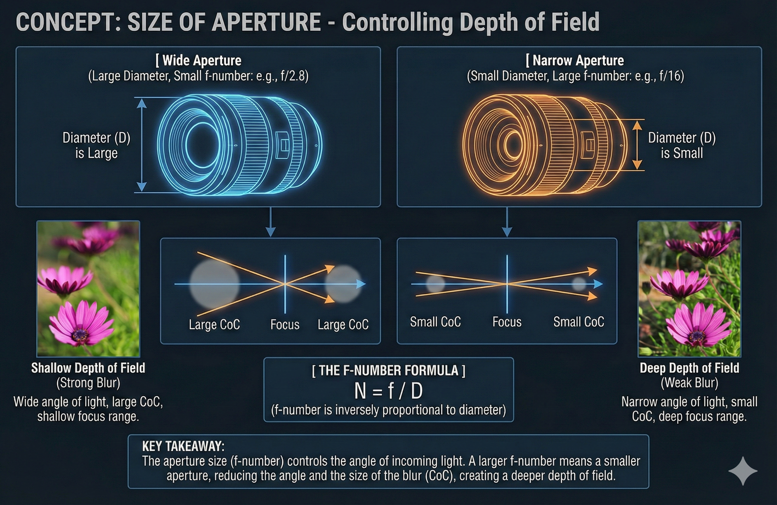
- The aperture, via its f-number, determines the degree of blur for objects outside this plane.
- When the f-number increases, the aperture diameter decreases.
- This reduces the angle at which light rays enter the lens, thereby shrinking the CoC.
- Consequently, objects at distances other than the focal distance appear less blurry.
- Conversely, when the f-number decreases, the aperture diameter increases.
- This widens the angle of incoming light, expanding the CoC and causing objects outside the focal distance to appear more blurry.
- When the f-number increases, the aperture diameter decreases.
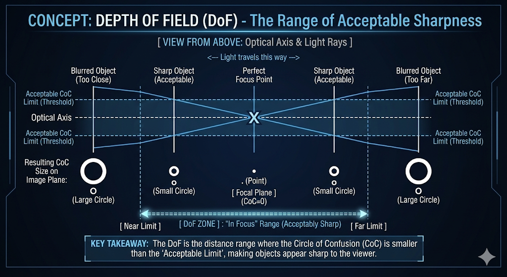
Depth of Field
- The depth of field (DoF) is the range of distances within a scene that appears acceptably sharp in an image.
- An object is considered “in focus” if the CoC formed by its reflected rays on the image plane is small enough to be perceived as a single point by the viewer.
- The size of the CoC depends on an object’s distance from the focal plane.
- A larger depth of field means a greater range of distances will appear in focus.
- This implies that even objects located significantly far from the focal distance may still appear acceptably clear, provided they remain within the boundaries of the DoF.
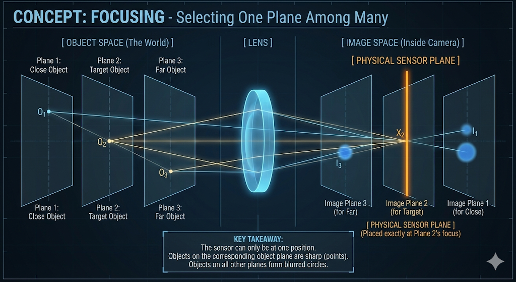
Focusing
- When a camera captures a scene, every object exists at a specific depth, or distance from the camera.
- Think of the world as being composed of numerous parallel object planes, each perpendicular to the camera’s view direction.
- Ideally, light rays originating from points on a single object plane would converge to a single corresponding image plane within the camera.
- This implies that each object plane has its own distinct image plane where its light rays would be in perfect focus.
- However, a camera’s sensor can only occupy a single, fixed image plane at any given moment.
- When this plane is selected for rendering, rays from objects on all other planes will not be in sharp focus.
- Instead of converging to a single point, these rays will intersect the selected image plane as a blurred disc known as the circle of confusion (CoC).
- The size of this circle determines the degree of blur for that specific point.
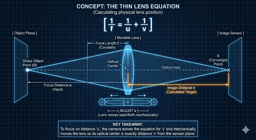
How to Choose the Image Plane
-
The camera determines the appropriate image plane to render by adjusting its internal optics, a process explained by the Thin Lens Equation:
\[{1\over f} = {1\over u} + {1\over v}\]- where
- $f$ is the focal length of the lens.
- $u$ is the focus distance, the distance from the lens to the object plane that is intended to be in perfect focus.
- $v$ is the image distance, the distance from the lens’s optical center to the image sensor or image plane.
- This is the variable that is physically adjusted to achieve focus.
- where
-
The Thin Lens Equation shows that for a given focal length ($f$), the image distance ($v$) is uniquely determined by the focus distance ($u$).
- Therefore, achieving focus on an object at a specific distance is accomplished by physically moving the lens assembly relative to the image sensor.
- This physical movement of the optical center ensures that rays from the desired object plane converge precisely onto the camera’s sensor, thus bringing that object into sharp focus.
Implementing Visual Effects
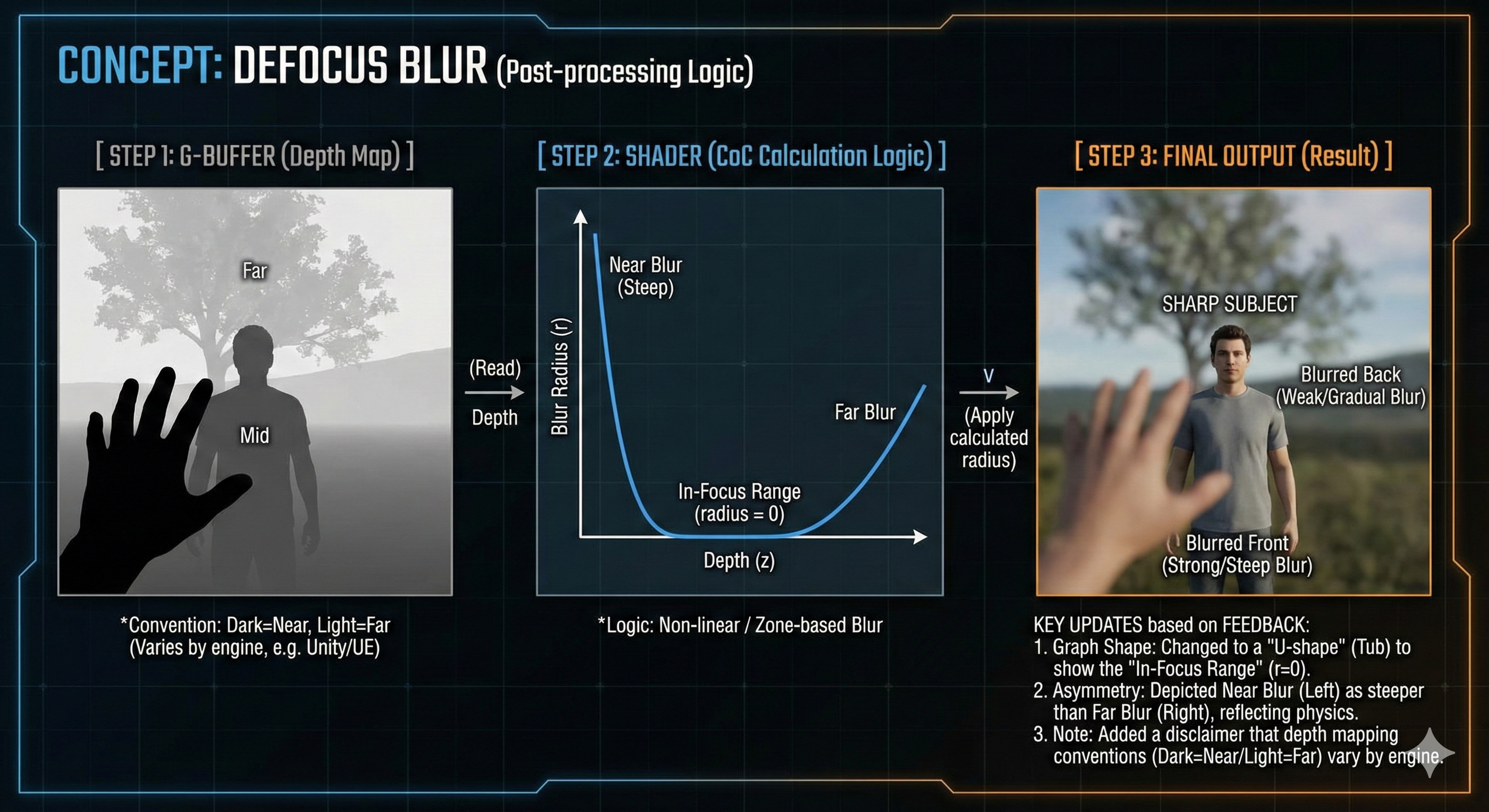
Defocus Blur (Depth of Field)
- Defocus blur, commonly known as Depth of Field (DoF), occurs when objects are not within the camera’s focus range, causing their CoC to become perceptibly large.
- In real-time rendering, simulating this physical process is computationally expensive.
- Therefore, a common alternative is a post-processing technique using a G-Buffer.
- A G-Buffer (Geometry Buffer) stores per-pixel data, including depth, position, and surface normals.
- A post-processing shader then uses this depth information to calculate a blur radius for each pixel based on its distance from the camera’s focal plane.
- If a pixel’s depth is within the DoF boundaries,
- its Circle of Confusion (CoC) radius is set to zero (meaning no blur).
- If a pixel’s depth is outside the boundaries,
- the shader calculates a blur radius.
- This radius is scaled based on how far the pixel’s depth is from the in-focus boundaries.
- The further a pixel is from the plane of focus, the larger the calculated blur radius will be.
- If a pixel’s depth is within the DoF boundaries,
- A post-processing shader then uses this depth information to calculate a blur radius for each pixel based on its distance from the camera’s focal plane.
-
Pixels within the DoF receive little to no blur, while pixels outside of it are blurred according to their distance from the focal plane, simulating the defocus effect.
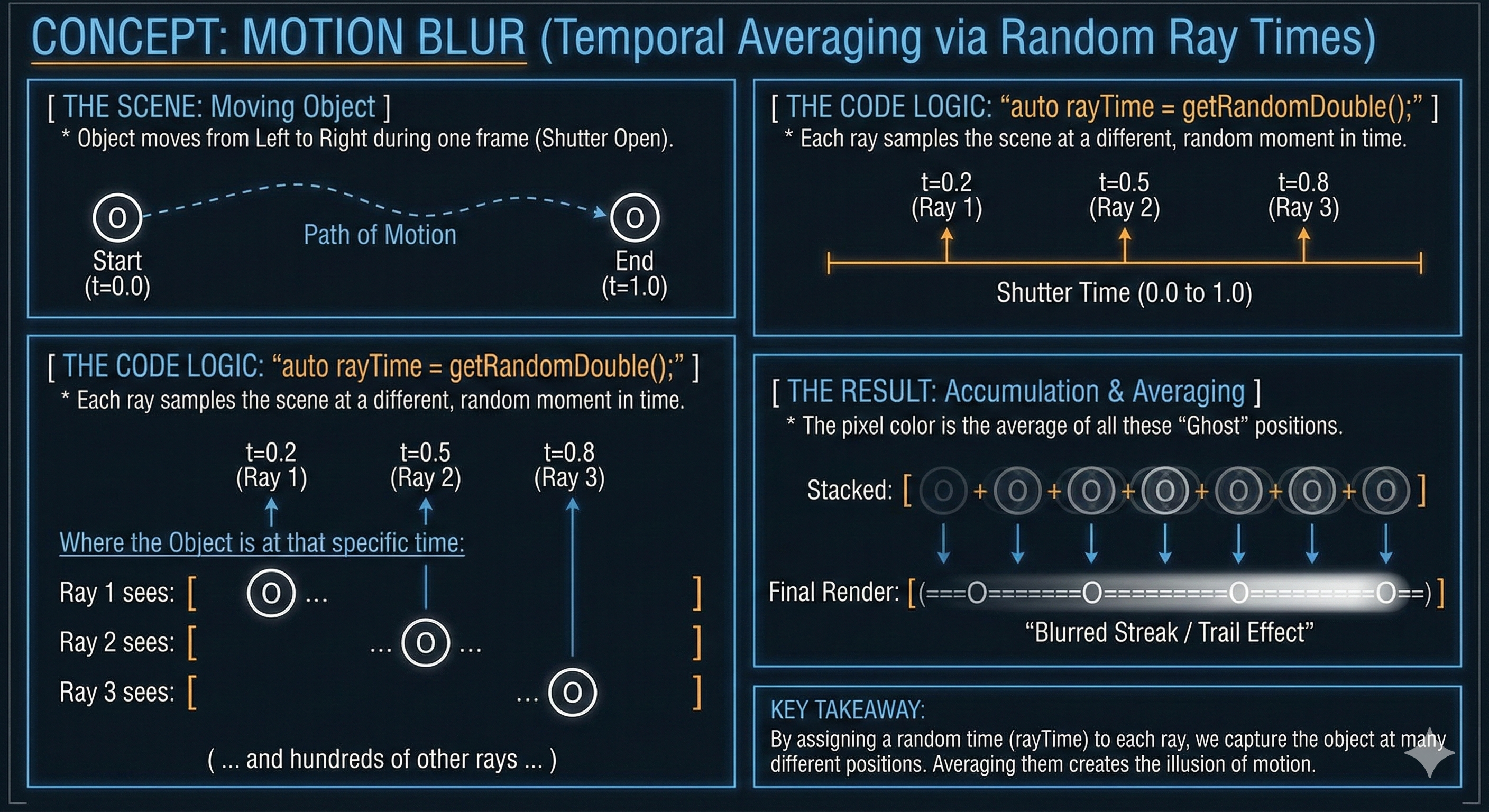
Motion Blur
- Motion blur is an effect that simulates the streaking of objects in motion, as a result of a short exposure time.
- This is implemented by averaging the color of a pixel across multiple frames or time steps, similar to how defocus blur is achieved by averaging samples across a spatial area.
-
The final color of a pixel is a blend of its colors at different moments in time, creating the illusion of motion.
-
Click to see the code
  Ray getRayToSample(int currentWidth, int currentHeight) const {
      auto offset = getSampleSquare();
      auto pixelSample = pixelCenterTopLeft
          + ((currentWidth + offset.getX()) * pixelDeltaWidth)
          + ((currentHeight + offset.getY()) * pixelDeltaHeight);

      auto rayOrigin = (defocusAngle <= 0) ? center : getDefocusRandomPoint();
      auto rayDirection = pixelSample - rayOrigin;
      auto rayTime = getRandomDouble();

      return Ray(rayOrigin, rayDirection, rayTime);
  }
Primitive Intersection: The Cost of Scene Traversal
- After the camera generates a ray, the most critical operation is determining where and if that ray intersects any geometric primitives in the scene.
- While simple shapes like spheres and triangles have straightforward intersection tests, complex primitives, such as the quadrilateral, demand multi-step analytical geometry.
- A quadrilateral (quad) intersection requires a two-step process to ensure robust geometry handling, combining a Ray-Plane test with a subsequent boundary check.
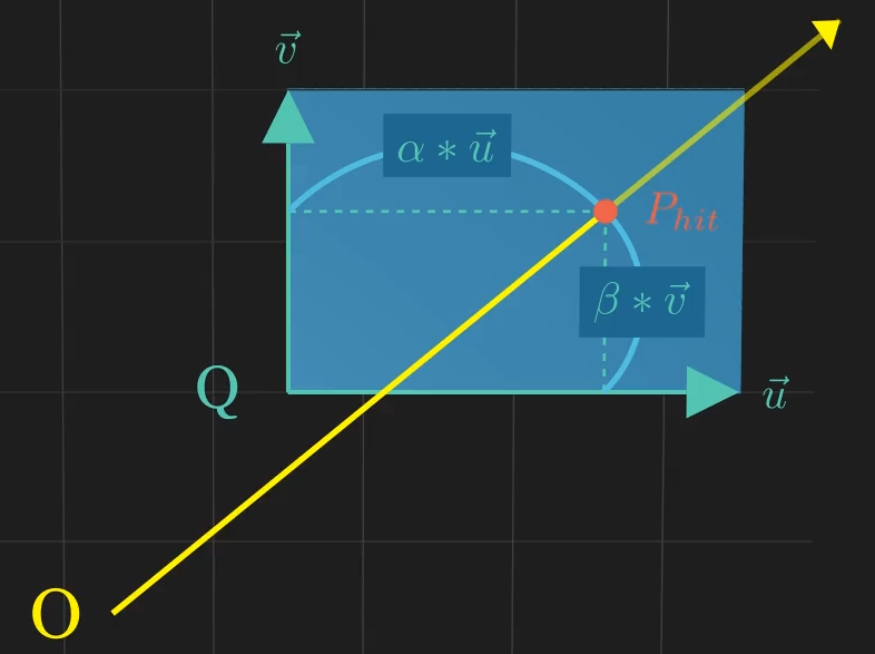
Quad Definition
- A quad is defined parametrically by a starting point $\mathbf{Q}$ and two direction vectors $\vec{u}$ and $\vec{v}$. Any point $\mathbf{P}(i, j)$ on the infinite plane is:
- The quad itself is the constrained region where $\mathbf{0 \le i \le 1}$ and $\mathbf{0 \le j \le 1}$.
The Two-Step Intersection Logic
- Ray-Plane Intersection (Time $t$): Find the intersection point $\mathbf{P_{hit}}$ on the infinite plane containing the quad by solving the combined Ray and Plane equations for $t$.
- Point Containment Check (Parameters $\alpha, \beta$): Ensure that the intersection point $\mathbf{P_{hit}}$ lies within the quad’s defined boundaries by calculating the parameters $\alpha$ and $\beta$ and checking if they are between 0 and 1.
-
Success Condition: The ray hits the quad if $\mathbf{t \ge 0}$ and $\mathbf{0 \le \alpha \le 1}$ and $\mathbf{0 \le \beta \le 1}$.
Anti-Aliasing
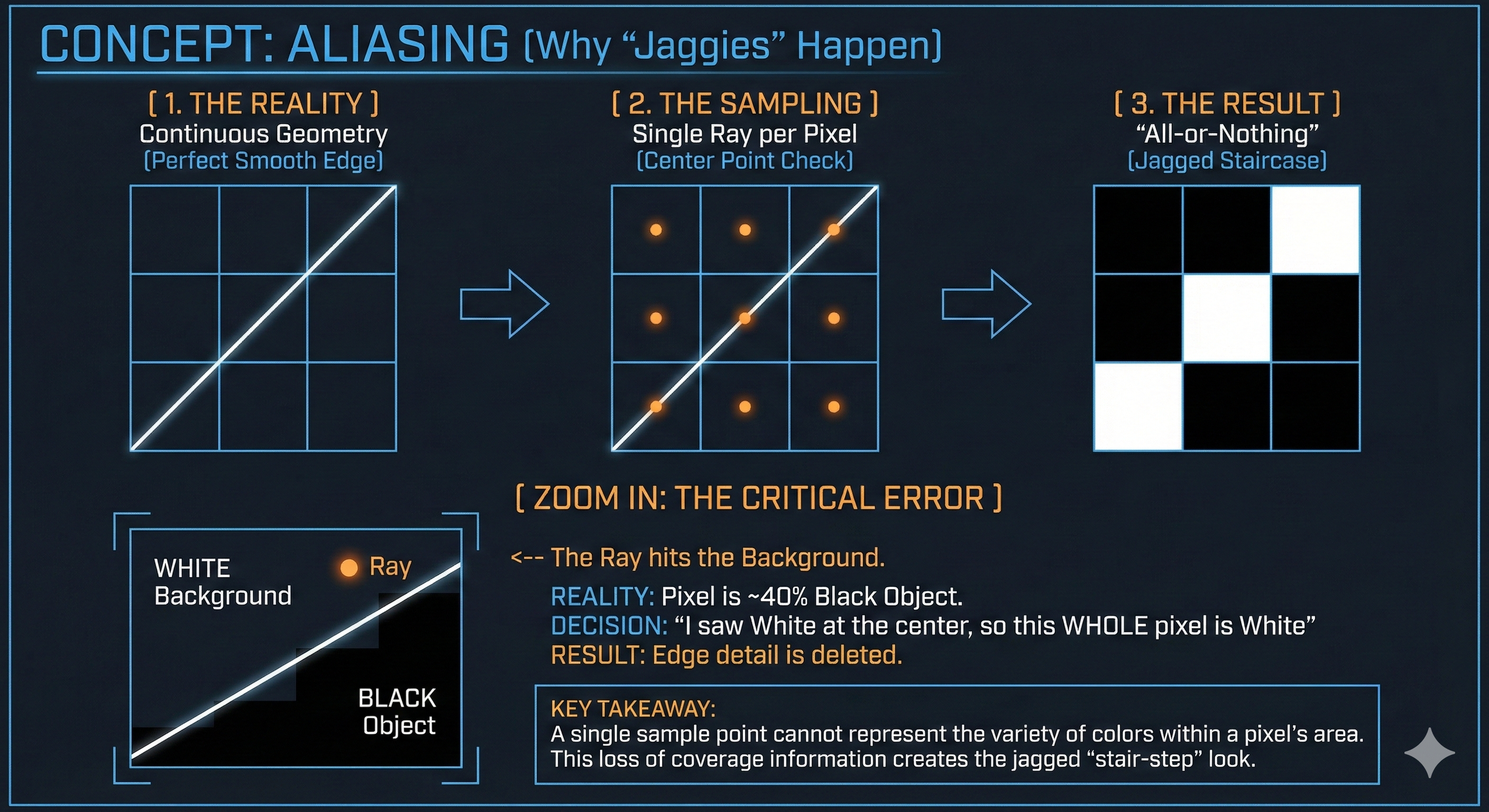
- Aliasing is a common visual problem in computer graphics where sharp edges and lines appear jagged or “stair-stepped.”
- This happens because a continuous, smooth 3D scene is projected onto a discrete grid of pixels on a screen.
- Each pixel can only display a single, solid color. The core reason for this issue is a process called point sampling.
Why Aliasing Occurs
- In ray tracing, the color of a pixel is traditionally determined by casting a single ray from the camera, through the center of the pixel, into the scene.
- The color of whatever the ray hits is then used for that entire pixel.
- The issue is that a single pixel represents a small square area of the scene, not just a single point.
- If a sharp edge—for instance, where a black object meets a white background—falls within that pixel’s area, the single ray cast to the center might only hit the white background.
- The black part of the edge is completely missed.
- This “all-or-nothing” approach leads to the loss of detail, causing the jagged stair-step appearance.
- A pixel’s color is determined by a single sample, but the area it represents may contain multiple colors in the scene.
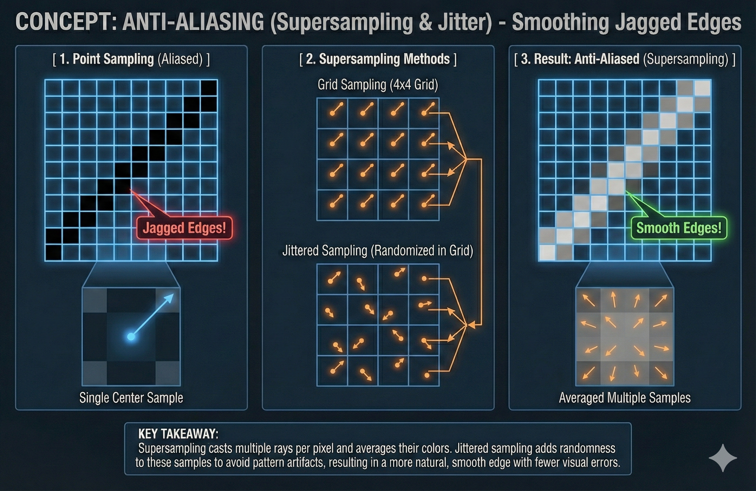
How to Fix
- The solution is to use supersampling, which involves casting multiple rays for each pixel instead of just one.
- The key idea is to sample different locations within the pixel’s area and then average the resulting colors to get a more accurate representation of the true color.
- This blending of colors smooths out the transitions between objects, eliminating the jagged edges.
- Supersampling methods differ in how they choose the multiple sample locations within each pixel:
- Grid Sampling
- The pixel is divided into a regular grid (e.g., 2x2, 4x4), and a ray is cast to the center of each sub-grid cell.
- For a 4x4 grid,
- 16 rays are cast
- and their average color value will be the color value of that cell
- For a 4x4 grid,
- This method is straightforward and effective but can sometimes miss fine details or produce its own visual artifacts if the sampling grid aligns with a repeating pattern in the scene.
- The pixel is divided into a regular grid (e.g., 2x2, 4x4), and a ray is cast to the center of each sub-grid cell.
- Jittered Sampling:
- This is a more advanced technique.
- It also divides the pixel into a grid, but instead of casting a ray to the center of each cell, it casts the ray to a randomly chosen point within each cell.
- This small bit of randomness helps prevent the structured artifacts of grid sampling while still ensuring that samples are distributed evenly across the pixel’s area.
- Jittered sampling produces a more natural and accurate result with fewer visible artifacts.
- This is a more advanced technique.
- Grid Sampling
Post-Processing & Final Display
- The final stage of the rendering pipeline involves processing the high-dynamic-range (HDR) image data—which contains light intensity values calculated in linear space—and transforming it into a perceptually correct, low-dynamic-range (LDR) image suitable for standard displays.
Tonemapping: Compressing the Dynamic Range
- Tonemapping is the vital process of mapping the wide range of luminance (brightness) values in a rendered HDR image down to the narrow range that a standard monitor can display.
- The Problem: Physically based rendering calculates light accurately, often resulting in extremely bright values (e.g., from direct sunlight) that exceed the $0$ to $1$ range of a standard LDR image file (like an 8-bit JPEG).
- Displaying these values without adjustment would clip the highlights, resulting in loss of detail.
- The Solution: A tonemapping operator applies a non-linear curve to compress the bright parts of the image while preserving the details in the mid-tones and shadows.
- Two widely used operators are:
- Reinhard Operator: A simple, computationally cheap operator that models a photographic exposure process.
- It compresses highlights smoothly but can sometimes result in a somewhat flat or washed-out look:
- Where $L_{in}$ is the linear input luminance and $L_{out}$ is the resulting LDR luminance.
- ACES (Academy Color Encoding System): A more sophisticated, filmic tonemapping standard known for its vibrant look and excellent preservation of color saturation, particularly in highlights.
- It uses a complex curve derived from cinematic color science to produce a result that visually resembles a high-quality film stock.
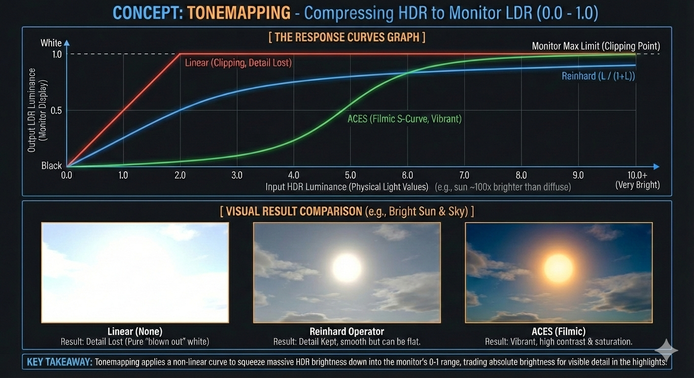
- Reinhard Operator: A simple, computationally cheap operator that models a photographic exposure process.
Color Transformation and Look-Up Tables (LUTs)
- After tonemapping, the image undergoes a Color Transformation to apply specific artistic styles or correct color imbalances. This is often done using a Look-Up Table (LUT).
- Purpose: A LUT is a pre-calculated data set used to quickly modify the color of a pixel based on its original RGB values.
- Implementation: LUTs are often implemented as a $3\text{D}$ texture cube.
- The original RGB color of a pixel acts as the coordinate $(r, g, b)$ to sample the LUT cube.
- The value stored at that coordinate in the cube is the new, transformed RGB color.
- Efficiency: Applying a complex color grading operation (like changing contrast or white balance) through a LUT involves a single texture lookup operation per pixel, making it significantly faster than executing a lengthy mathematical function for every pixel.

Gamma Correction (Display Output)
- As established in Post 1, the final, tonemapped LDR image must be converted from Linear Space back to Gamma Space (sRGB) before being sent to the monitor.
- This final transformation ensures that the image is perceptually balanced, accounting for the non-linear response of display hardware, which makes the image appear correct to the human eye.
Leave a comment