Computer Graphics: Textures

한국어

Textures

• In computer graphics, Texture Mapping is the process of applying material effects onto a geometric shape (Geometry), serving as a core technique to enhance the realism of 3D objects.
• This section comprehensively covers topics from the basic methods of texture mapping to Perlin Noise , a procedural texture generation technique, and Shadow Mapping for providing depth and realism.

Texture Mapping

Texture mapping is broadly classified into three methods based on their dependence on the coordinate system.

Types of Mapping

• Constant Texture:
  • Concept: Returns a single, uniform color value for all points, regardless of the surface position or object movement.
  • Feature: The simplest form, independent of spatial coordinates or geometric information. (e.g., a solid red sphere)
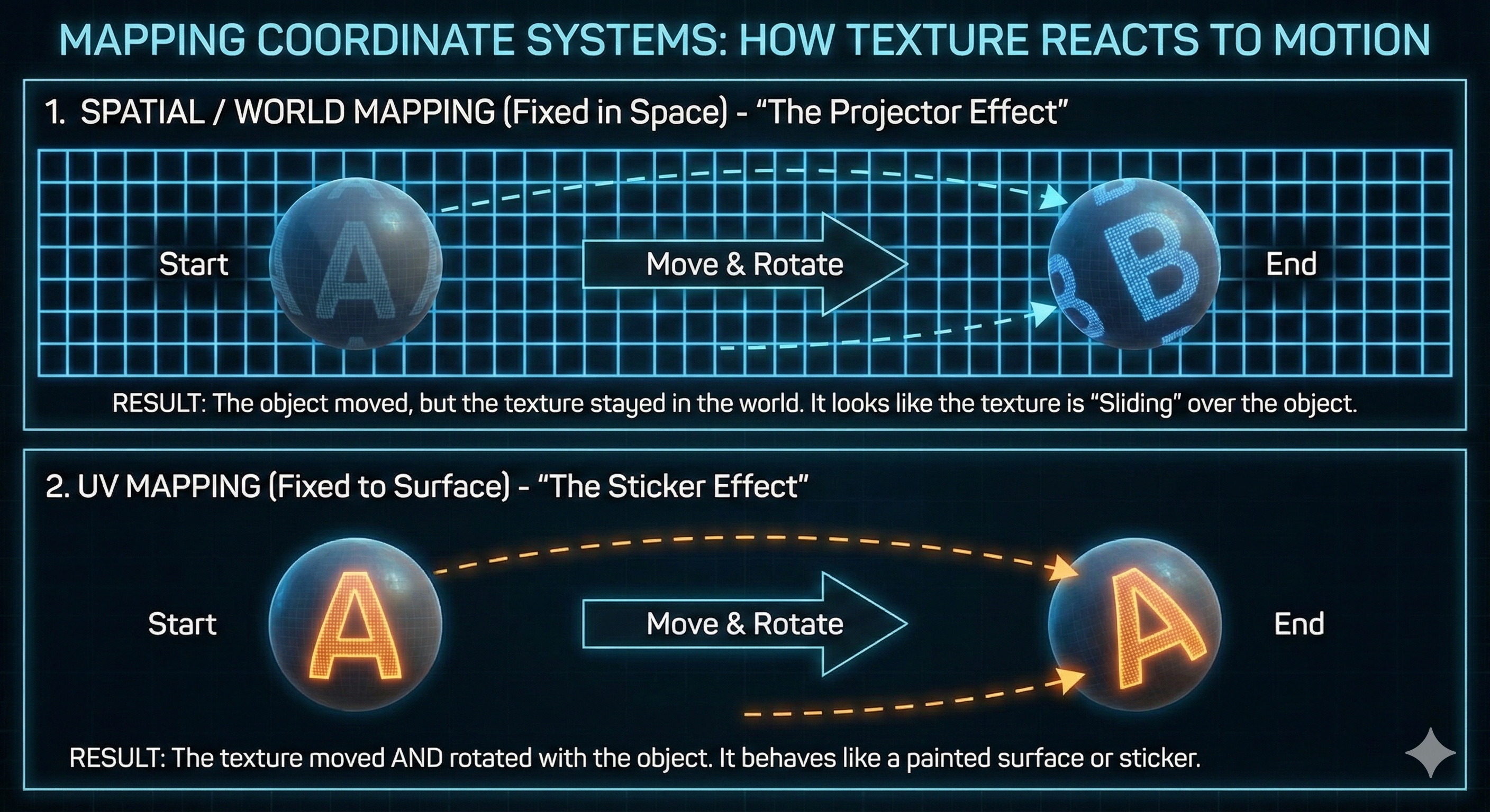
• Spatial/World Space Texture:
  • Concept: The texture is defined based on coordinates in 3D world space, not on the object’s surface.
  • Feature: Since the texture is fixed to an absolute position in space, if the object moves or rotates, the texture will slide or distort on the surface instead of moving along with it. This is similar to a projected image remaining fixed on a wall even if the wall moves.
• UV-Mapped Texture:
  • Concept: The most common 3D texturing method. It explicitly links the object’s geometric surface with the texture image using a 2D coordinate system ($U, V$).
  • Feature: Each vertex is assigned unique $(u, v)$ coordinates, ensuring the texture “sticks” to the surface and moves along with the object when it translates or rotates, maintaining its unique appearance. (e.g., a logo on a T-shirt)

  

Procedural Texture

This method generates textures using only mathematical algorithms without image files. It offers advantages in memory efficiency and lack of resolution constraints.

Checkerboard Texture

• Core Principle: Utilizes the $x, y, z$ coordinates of the ray’s hit point. The color is alternated by performing an integer operation (Modulo 2) on the sum of the floor of each coordinate.

• Implementation Formula: The size of the grid can be controlled by dividing each coordinate by a specific constant ($scale$).

  \[\text{Pattern} = \left( \left\lfloor \frac{p_x}{scale} \right\rfloor + \left\lfloor \frac{p_y}{scale} \right\rfloor + \left\lfloor \frac{p_z}{scale} \right\rfloor \right) \bmod 2\]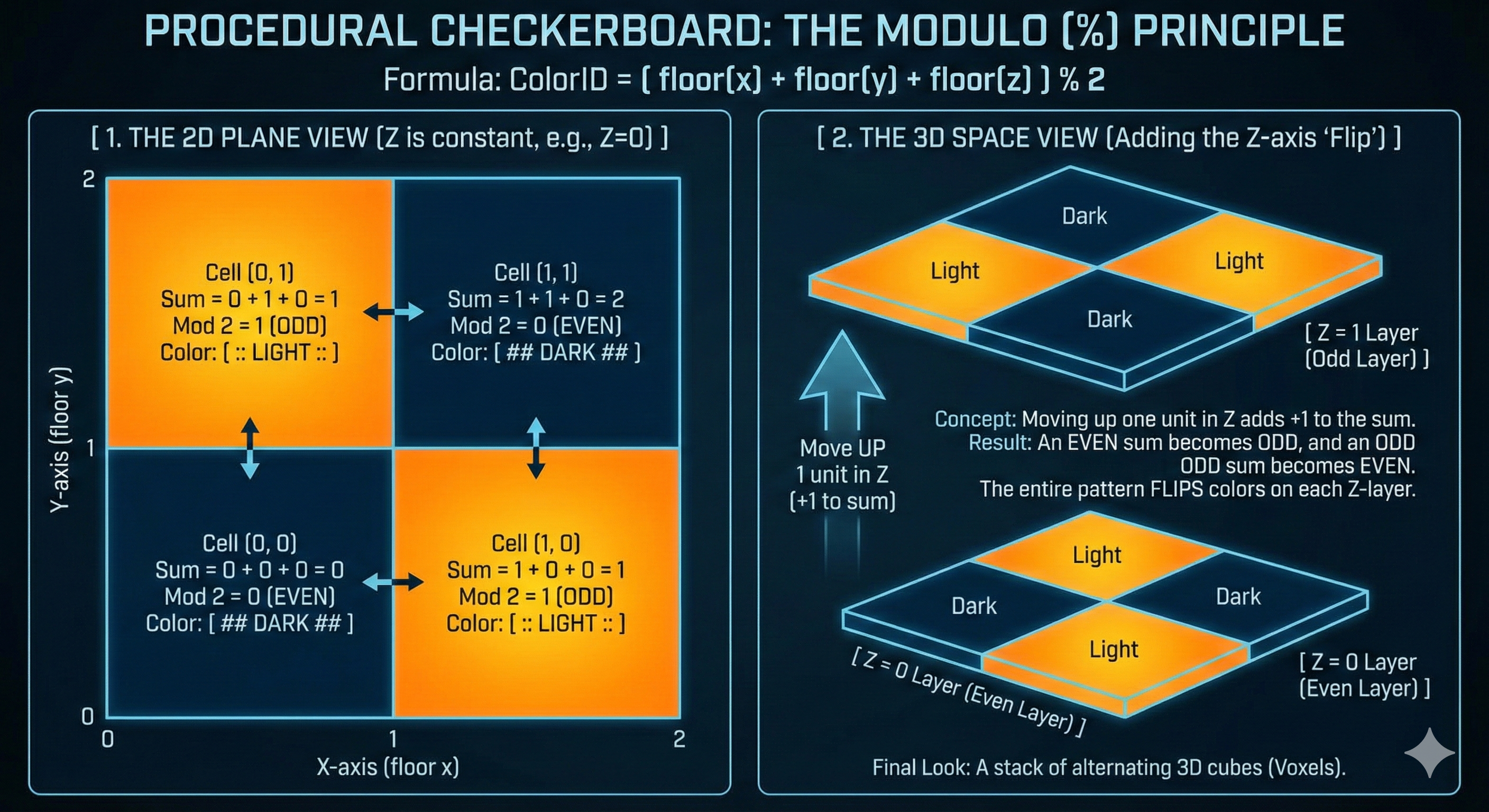

  

Detailed Analysis of Perlin Noise

• Perlin Noise is a procedural texture algorithm that generates Deterministic Random Values, creating smooth, continuous patterns that exhibit randomness.
• It is primarily used to simulate the organic irregularity of natural phenomena like clouds, fire, and terrain.

Core Concepts and Features

• Definition: Generates deterministic random values, guaranteeing the same output for the same input coordinates ($x, y, z$).
• Characteristic: The output value changes very smoothly and organically as the input position changes.
• Pattern Size: The size of the user-defined Permutation Table (P-Table) determines the repetition period of the noise pattern. For example, if the table size is $2^8$, unique random values are only generated in the range $0 \sim 255$, after which the pattern repeats.
• Efficiency: The core table containing the basic noise pattern is generated only once at the beginning, reducing the computational load as complex random number calculations don’t need to be performed every frame.

Basic Operating Principle (Multiple Random Application)

Perlin Noise applies and combines ‘randomness’ over multiple stages to create predictable yet complex patterns.

1. Permutation Table Generation: A sequence of integer values (e.g., $0 \sim 255$) is arranged and the order of elements is randomly shuffled to create the Permutation Table (P-Table). This table provides the fixed pattern.
2. Coordinate Hashing (Truncation): The input position value (e.g., the $x$ coordinate) is converted (Truncated) into a valid table index by performing an AND operation ($\& 255$) with the table size (e.g., 255).
3. Random Value Extraction and Combination: The index is used in the P-Table to retrieve a random value. This process is performed for each axis ($x, y, z$), and the resulting multiple random values are combined (e.g., using an XOR operation) to obtain the final random value.

Detailed Implementation Steps (Grid Points and Interpolation)

The core of Perlin Noise is divided into two steps: preparing grid point information and smooth interpolation.

Grid Point Information Preparation (Permutation Table & Gradient)

• Permutation Table (P-Table) and Gradient Vector Assignment:
  • P-Table Role: The core structure determining the basic noise pattern, typically created by shuffling an array of size $2^n$ (e.g., 256).
  • Gradient Vector ($G$): Each of the 8 corners (grid points) of the unit cube surrounding the input position $P$ is assigned a randomly oriented Unit Vector via the P-Table. This vector is the Gradient Vector.
• Influence Calculation (Dot Product):
  • Distance Vector ($D$): The relative distance vector from each grid point to the input position $P$ is calculated.
  • Dot Product: The Dot Product ($G \cdot D$) is calculated between the Gradient Vector ($G$) and the Distance Vector ($D$).
  • Meaning: This dot product represents the predicted gradient or influence from that grid point. As point $P$ approaches a specific grid point, the dot product approaches 0, which serves as the input value for interpolation.

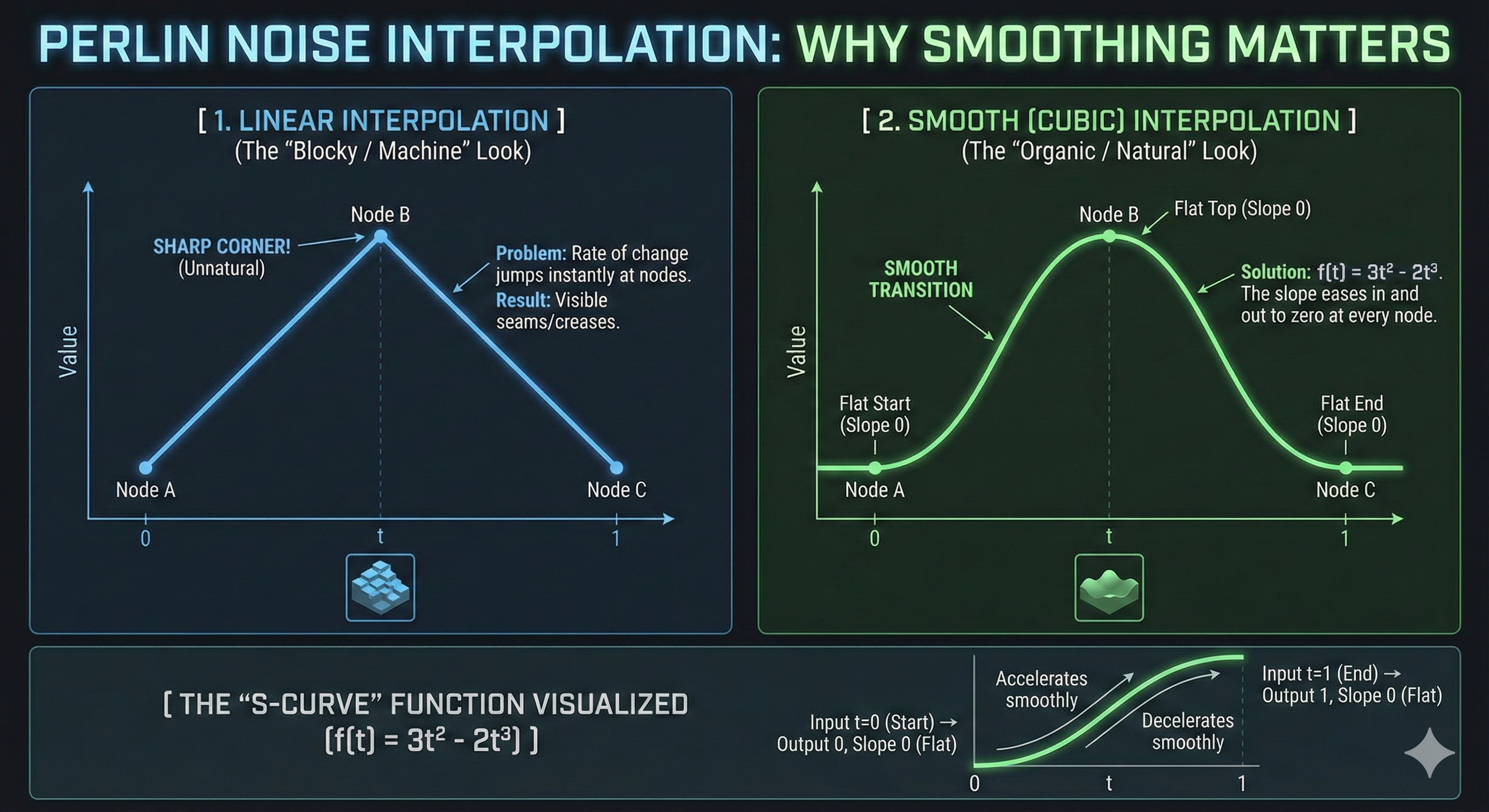
Smooth Interpolation (Interpolation & Smoothing)

• Smoothing Function:
  • Purpose: Using simple linear interpolation causes the noise gradient to change abruptly at grid boundaries, leading to unnatural seams or a blocky appearance.
  • Solution: A cubic smoothing function is applied to the fractional part of the input position $P$ ($t$, i.e., $u, v, w$). The most common formula is: \(f(t) = 3t^2 - 2t^3\)
  • Feature: This function ensures the derivative (slope) is 0 at $t=0$ and $t=1$, guaranteeing that the noise pattern connects smoothly at the grid points.

• Trilinear Interpolation: The 8 dot product values (influences) are interpolated (summed) using the smoothed weights ($u’, v’, w’$) in the order $X \rightarrow Y \rightarrow Z$ to obtain the final noise value. Since the sum of all weights is 1, the final value takes the form of a weighted average.

  

Mathematical Background of Hermite Smoothing

The cubic smoothing function used in Perlin Noise, $f(t) = 3t^2 - 2t^3$, is a special form of the Cubic Hermite Spline.

• Hermite Spline Definition: A spline controlled by specifying the position ($P_0, P_1$) and the derivative/slope ($M_0, M_1$) at both endpoints.
• Smoothing Function Derivation: The noise smoothing function is derived by setting the following conditions in the general Hermite Spline formula:
  • Start position $P_0 = 0$, End position $P_1 = 1$.
  • Start tangent $M_0 = 0$, End tangent $M_1 = 0$ (Slope is set to 0 at the boundaries).
  • Substituting this setting into the general formula yields the simple cubic function $p(t) = -2t^3 + 3t^2$ (or $3t^2 - 2t^3$).
• Meaning: This function creates an Ease-in/Ease-out effect where the rate of change is 0 near $t=0$ and $t=1$, making the start and end of the change smooth, thus resulting in natural noise interpolation.

Spherical Coordinate Transformation (Spherical Mapping)

Spherical coordinate transformation is a key technique in UV mapping used to map 3D space coordinates to the 2D coordinates of a texture image. It is essential for applying environment maps or regular textures to rotationally symmetric objects like a Sphere.

Basic Concept

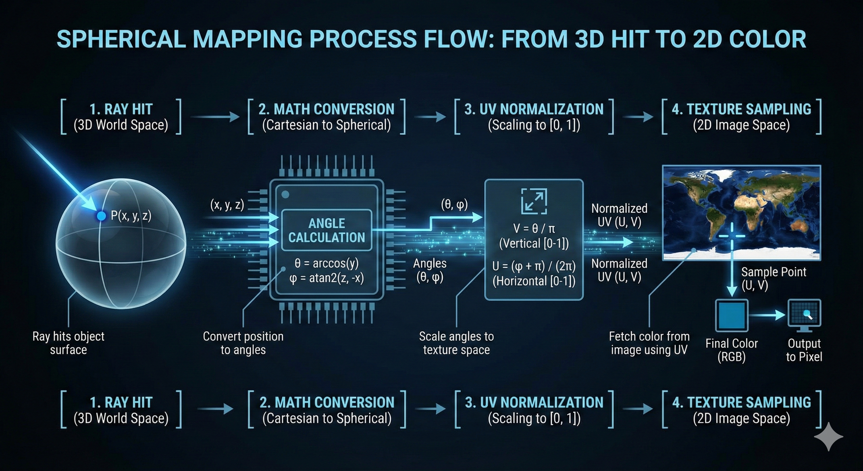
• Objective: To convert the 3D position where the ray hits ($P = (x, y, z)$) into the 2D texture image coordinates ($U, V$).
• Principle: This is based on the transformation between the Cartesian Coordinate System ($x, y, z$) and the Spherical Coordinate System ($r, \theta, \phi$). (Here, we assume the object is on a unit sphere, so $r=1$ is used.)
• Application: In ray tracing, when a ray hits an object, the ($x, y, z$) values of the hit point are converted into angular information ($\theta, \phi$) to fetch the corresponding color value from the texture image.

Coordinate System Definition and Derivation

Before deriving the transformation formulas, it is crucial to clearly define the coordinate system used, as this definition determines the signs in the final formulas.

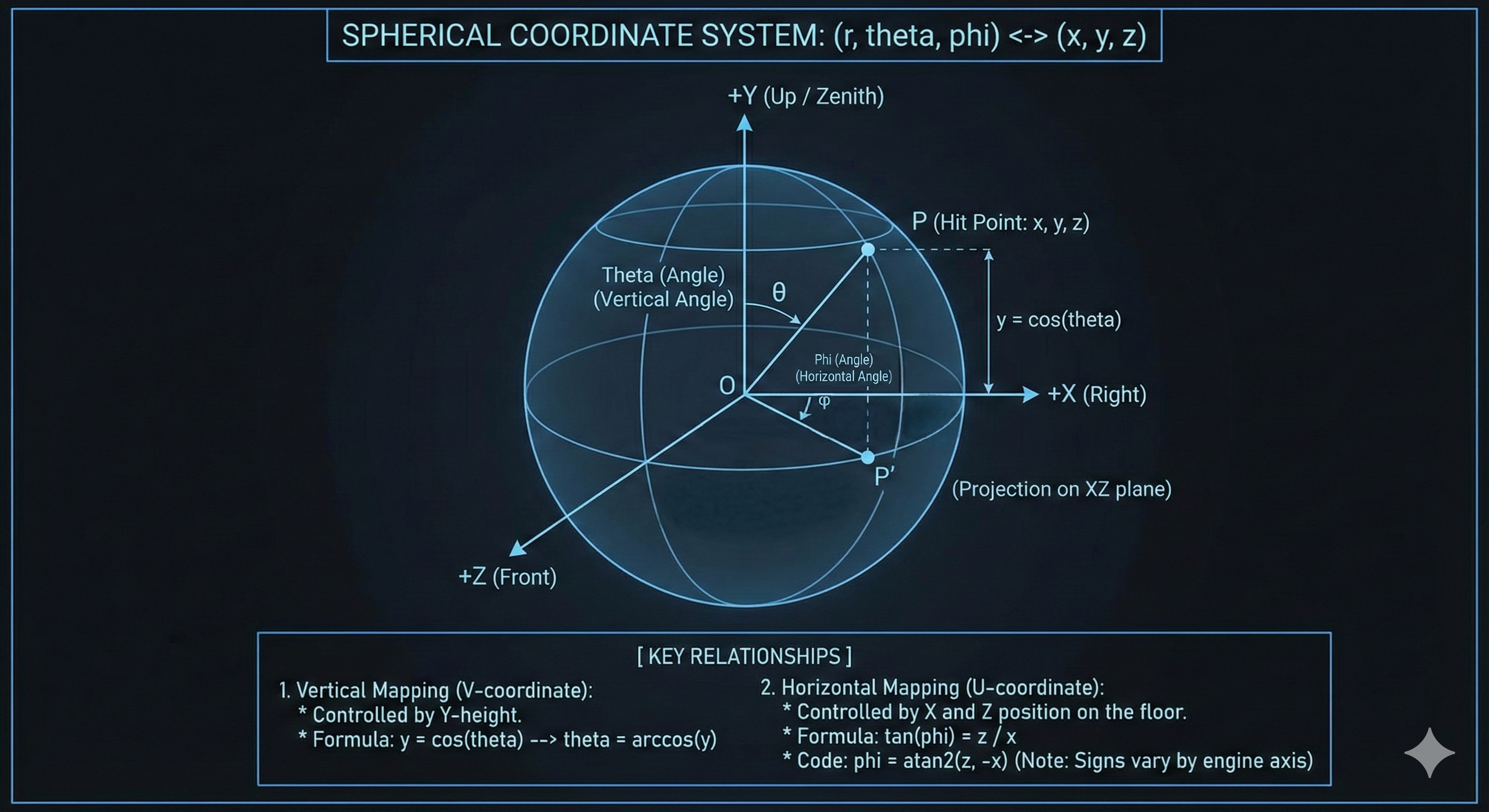
• Axis Definition:
  • $x$ (Left/Right): Right
  • $y$ (Up/Down): Up (zenith direction)
  • $z$ (Front/Back): Front
• Angle Definition:
  • $\theta$ (Vertical Angle): Angle descending from the $+y$ axis (Up) (polar angle, latitude)
  • $\phi$ (Horizontal Angle): Angle rotating from the $+x$ axis (Right) towards the $+z$ axis (Front) (azimuthal angle, longitude)

  

$x, y, z$ $\rightarrow$ $\theta, \phi$ Derivation

The transformation formula is generally derived by reversing the process of obtaining Cartesian coordinates from spherical coordinates ($(\phi, \theta) \rightarrow (x, y, z)$). (Assuming hypotenuse $r=1$)

• Deriving $\mathbf{\theta}$ from $\mathbf{y}$ coordinate (Vertical Component):
  • The $y$ value is easily found using the hypotenuse (radius) and the vertical angle $\theta$.
  \[y = \cos\theta\]
  • Therefore, $\theta$ is obtained through the $\arccos$ function.
  \[\theta = \arccos(y)\]
• Deriving $\mathbf{x, z}$ coordinates (Horizontal Component): When point $P$ is projected onto the $xz$ plane, the distance between the origin and the projected point is $\sin\theta$. This distance is used as the hypotenuse to derive $x$ and $z$.

  • $\mathbf{x}$ Derivation:

    \[\cos\phi = \frac{x}{\sin\theta} \implies x = \sin\theta \cos\phi\]

  • $\mathbf{z}$ Derivation:

    \[\sin\phi = \frac{z}{\sin\theta} \implies z = \sin\theta \sin\phi\]

  • The $\phi$ angle is derived using the $\tan$ relationship between $x$ and $z$.

    \[\tan\phi = \frac{\sin\phi}{\cos\phi} = \frac{z/r}{x/r} = \frac{z}{x}\]

  • Therefore, $\phi$ is obtained using the $\operatorname{atan2}$ function. $\operatorname{atan2}$ takes two variables ($y, x$) and returns the correct angle considering the quadrant.

    \[\phi = \operatorname{atan2}(z, -x)\]

Final Transformation Formulas

• Given the hit position $P(x, y, z)$, the angles $\theta$ and $\phi$ corresponding to the texture coordinates are:

\[\theta = \arccos(y) \quad (\text{corresponds to Vertical coordinate, } V)\] \[\phi = \operatorname{atan2}(z, -x) \quad (\text{corresponds to Horizontal coordinate, } U)\]

• These angle values are then normalized to the range of the $V$ (vertical) and $U$ (horizontal) coordinates (e.g., $[0, 1]$ or $[0, \text{number of texels}]$) and used to sample the 2D image texture.

  

Implementation Considerations

• Coordinate System Consistency: The formulas above are based on defining $+y$ as Up. If the rendering system defines $+z$ as Up or uses different axes, the variables used in $\arccos$ and the variables and sign (e.g., $-x$) in $\operatorname{atan2}$ must be appropriately changed to match that convention.
• UV Coordinate Origin: Most image formats define the top-left corner as $(0, 0)$, but the origin’s position (e.g., bottom-left) can vary depending on the definition of a specific texture or environment map. This origin must be confirmed before applying the final texture coordinates.

Shadow Mapping

Shadow Mapping is a technique that utilizes depth information from the light source’s viewpoint to determine if an object is occluding another, thereby casting a shadow.

Core Principle of Shadow Mapping

The Shadow Mapping process consists of two main stages. The core concept is that Depth is defined relative to a specific Direction.

Stage 1: Shadow Map Generation (Depth Recording)

• Light View Rendering: The scene is rendered from the light source’s position and view. This operates conceptually similar to casting Shadow Rays from the light in all directions.
• Depth Storage: For each rendered pixel, the shortest distance to the first hit from the light source is measured. This distance is the Depth, and these values are stored in a 2D texture called the Shadow Map.
  • Directional Definition: The depth value stored in each texel of the Shadow Map represents the distance to the closest object in the specific direction corresponding to that texel’s position, as viewed from the light.

Stage 2: Shadow Determination (Depth Comparison)

When rendering the scene from the camera’s viewpoint, whether each point $P$ is in shadow is determined as follows:

• Transformation to Light Space:
  • The world coordinates of the rendering target point $P$ are transformed into Light Space coordinates using the light’s view and projection matrices.
  • Conceptual Meaning: This spatial transformation maps point $P$ to the same texel location in the Shadow Map as if it were viewed from the light source. That is, all points lying along the same direction emanating from the light will sample the same texel in the Shadow Map.
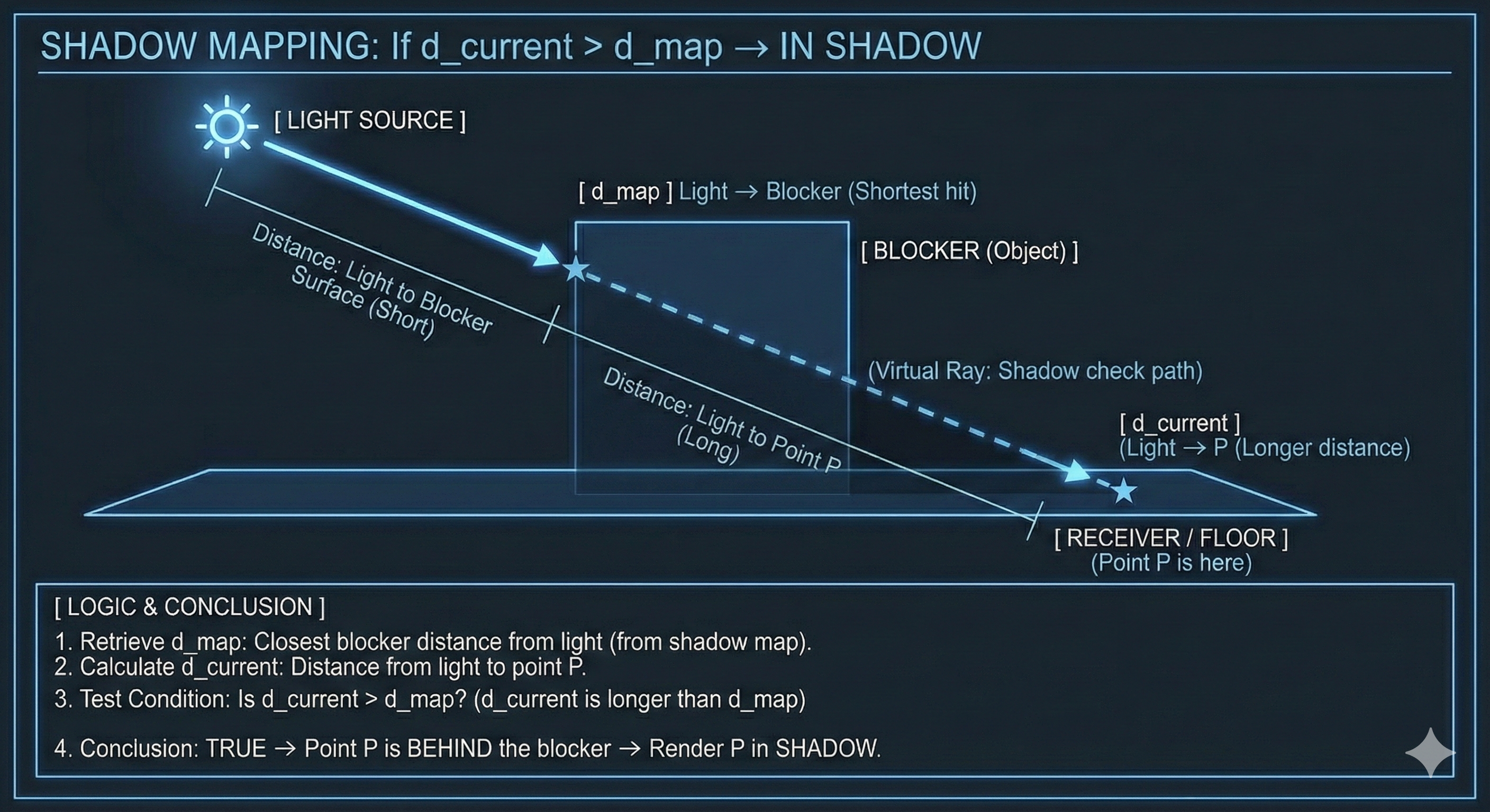
  • Lookup: The stored depth value ($d_{map}$) is looked up from the Shadow Map using the transformed Light Space coordinates.
• Distance Comparison:
  • Current Depth Calculation: The actual distance from point $P$ to the light source ($d_{current}$) is calculated, or the depth component ($z$ value) is extracted from the Light Space transformation result.
  • Determination:
    • $\mathbf{d_{current} > d_{map}}$: This means the distance from the current point $P$ to the light source is greater than the minimum depth stored in the Shadow Map. This implies there is another object (Obstacle) between $P$ and the light, and the light ray is occluded, thus a shadow is cast.
    • $\mathbf{d_{current} \approx d_{map}}$: If the distances are nearly equal, it means point $P$ is on the surface of the object closest to the light, so no shadow is cast.

  

Shadow Acne and Solution

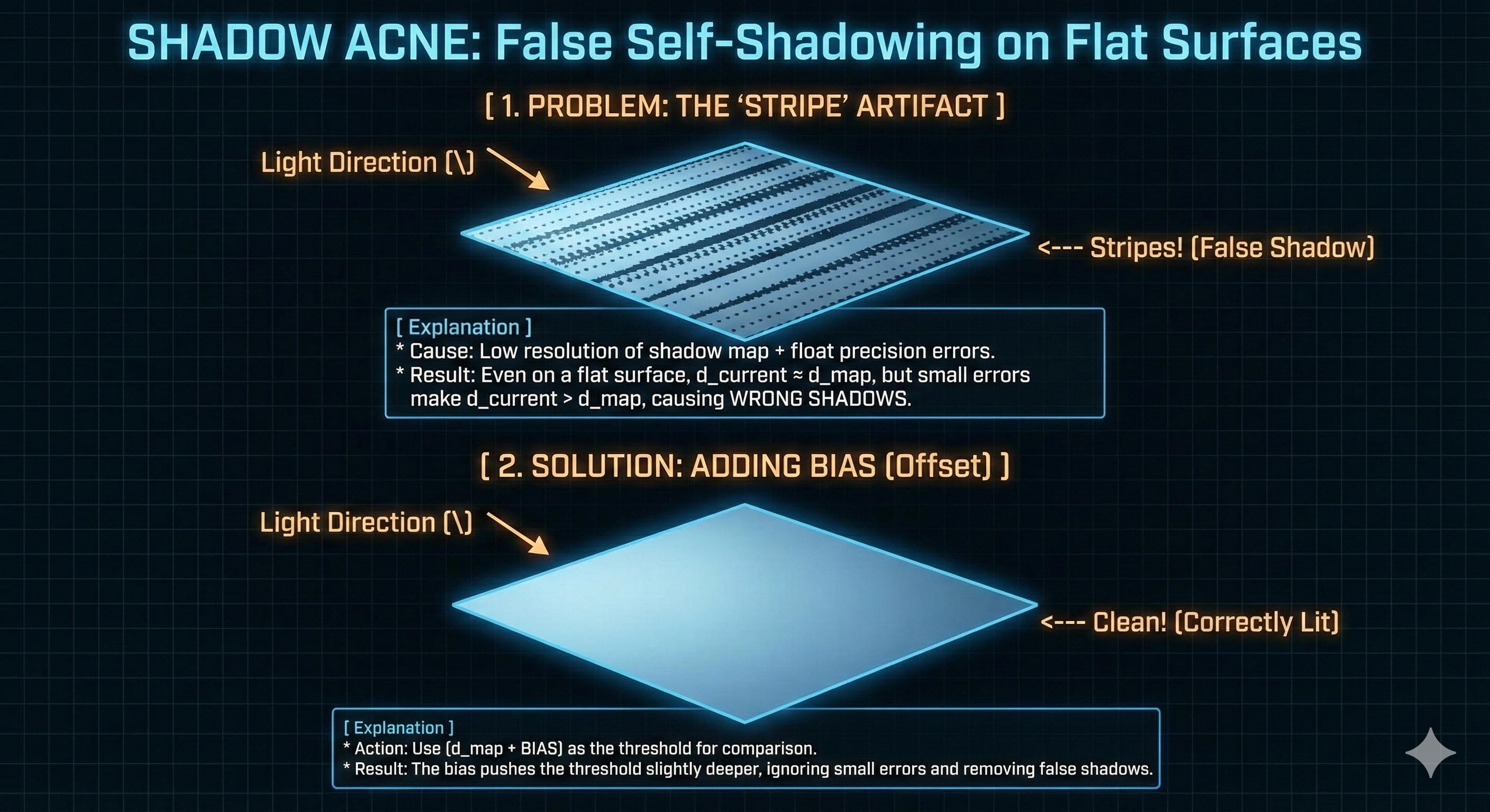
Shadow Acne is an unavoidable issue that occurs when implementing Shadow Mapping with floating-point numbers.

• Problem Cause: Due to the precision limits of floating-point arithmetic, a slight discrepancy error occurs where the stored depth ($d_{map}$) and the calculated current depth ($d_{current}$) in Stage 2 do not exactly match. This error can cause a surface that should be lit to be incorrectly judged as self-occluded, resulting in dark splotches (acne) on the surface.

• Solution (Bias): To correct this error, a very small positive value, Epsilon ($\epsilon$), is added to $d_{current}$ when comparing it with $d_{map}$ ($\mathbf{d_{current} + \epsilon}$). This offset slightly moves the ray’s starting point off the surface, preventing the misjudgment of Self-Intersection.

  

Top